
Transfer Learning for Image Classification
Image classification is one of the areas of deep learning that has developed very rapidly over the last decade. However, due to limited computation resources and training data, many companies found it difficult to train a good image classification model. Therefore, one of the emerging techniques that overcomes this barrier is the concept of transfer learning.
- What is Transfer Learning?
- Implementation
- Dataset
- Import libraries
- Defining data generators
- Define a callback to stop training after certain performance is achieved
- Define function to plot result
- Simple Convolutional Neural Network
- Transfer Learning using Inception v3
- Download model weights, import model, load weights into model
- Set layers to be non-trainable for pre-trained model
- Model summary of Inception v3
- Obtain last layer output of the pre-trained model
- Adding dense layers after pre-trained model
- Model summary of Inception v3 with dense layers
- Fitting the model
- Plotting model training and validation result
- Remarks
- Reference
What is Transfer Learning?
Transfer learning involves taking a pre-trained model, extracting one of the layers, then taking that as the input layer to a series of dense layers. This pre-trained model is usually trained by institutions or companies that have much larger computation and financial resources. Some of these popular trained models for image recognition tasks are VGG, Inception and ResNet.
Using this newly formed model, we can then set the parameters within the pre-trained model to be non-trainable while only optimizing the parameters of the subsequent dense layers during training.
✅ Due to limited computation resources and training data, many companies found it difficult to train a good image classification model
In order to illustrate the value of transfer learning, I will be comparing a simple convolutional neural network model against a model that utilises transfer learning in the following examples.
Implementation
The following sections will be focusing on implementation using Python.
Dataset
Before I go into the comparison, I will like to introduct you to the Fashion MNist dataset. This dataset consist of 10 different apparel classes, each of them is a 28x28 grayscale image. Fashion MNist was created to test the performance of categorical image classifier, making it ideal for the task that we are trying accomplish.
Note that you will have to download the images as PNG files for the following examples. Please refer to this repository for the steps to obtain the dataset.
Import libraries
Let’s start off by importing the necessary libraries
import os
import tensorflow as tf
from tensorflow.keras.optimizers import RMSprop
from tensorflow.keras import layers
from tensorflow.keras import Model
from tensorflow.keras.preprocessing.image import ImageDataGenerator
from tensorflow.keras.utils import plot_model
from tensorflow.keras import backend as K
import matplotlib.pyplot as plt
Defining data generators
train_dir = 'data/train'
validation_dir = 'data/test'

train_datagen = ImageDataGenerator(rescale=1./255,
                                   rotation_range=40,
                                   width_shift_range=0.2,
                                   height_shift_range=0.2,
                                   zoom_range=0.2,
                                   shear_range=0.2,
                                   horizontal_flip=True,
                                   fill_mode='nearest')  # with data augmentation for train set

valid_datagen = ImageDataGenerator(rescale=1./255)  # no augmentation for validation set

train_generator = train_datagen.flow_from_directory(train_dir,
                                                    batch_size=100,
                                                    class_mode='categorical',
                                                    target_size=(150, 150))


validation_generator = valid_datagen.flow_from_directory(validation_dir,
                                                         batch_size=100,
                                                         class_mode='categorical',
                                                         target_size=(150, 150))
Define a callback to stop training after certain performance is achieved
class myCallback(tf.keras.callbacks.Callback):
    def on_epoch_end(self, epoch, logs={}):
        if(logs.get('acc') > 0.99 and logs.get('val_acc') > 0.99):
            print("\nCancelling training as model has reached 99% accuracy and 99% validation accuracy!")
            self.model.stop_training = True
Define function to plot result
def plot_result(history):
    acc = history.history['accuracy']
    val_acc = history.history['val_accuracy']
    loss = history.history['loss']
    val_loss = history.history['val_loss']

    epochs = range(len(acc))

    plt.plot(epochs, acc, 'r', label='Training accuracy')
    plt.plot(epochs, val_acc, 'b', label='Validation accuracy')
    plt.title('Training and validation accuracy')
    plt.legend(loc=0)
    plt.figure()
    plt.show()
Simple Convolutional Neural Network
For the simple CNN model, I will be having 3 convolutional layers followed by a single dense layer and the output layer.
Defining CNN model
img_width, img_height = 150, 150

if K.image_data_format() == 'channels_first':
    input_shape = (3, img_width, img_height)
else:
    input_shape = (img_width, img_height, 3)

inputs = layers.Input(shape=input_shape)

x = layers.Conv2D(32, (2, 2), activation='relu')(inputs)
x = layers.MaxPooling2D(pool_size=(2, 2))(x)

x = layers.Conv2D(32, (2, 2), activation='relu')(x)
x = layers.MaxPooling2D(pool_size=(2, 2))(x)

x = layers.Conv2D(64, (2, 2), activation='relu')(x)
x = layers.MaxPooling2D(pool_size=(2, 2))(x)

x = layers.Flatten()(x)

x = layers.Dense(1024, activation='relu')(x)
x = layers.Dropout(0.2)(x)

outputs = layers.Dense(10, activation='softmax')(x)

model = Model(inputs=inputs, outputs=outputs)

model.compile(optimizer=RMSprop(lr=0.0001),
              loss='categorical_crossentropy',
              metrics=['accuracy'])
Model summary
model.summary()
plot_model(model, to_file='cnn_model.png', show_shapes=True, show_layer_names=True)
Fig. 1. CNN Model Architecture
Fitting the model
callbacks = myCallback()
history = model.fit_generator(generator=train_generator,
                              validation_data=validation_generator,
                              steps_per_epoch=100,
                              epochs=10,
                              validation_steps=100,
                              verbose=2,
                              callbacks=[callbacks])
Plotting model training and validation result
plot_result(history)
Fig. 2. CNN Model Result
Using a simple CNN model, we are able to achieve a validation accuracy of 0.7 after 10 epochs. Can we do better using transfer learning?
Transfer Learning using Inception v3
Inception is a convolutional neural network architecture introduced by Google which achieved top results in ImageNet Large Scale Visual Recognition Challenge 2014.
Fig. 3. Inception V3 - (Image source: here)
Download model weights, import model, load weights into model
# Download Inception v3 weights to local machine
!wget --no-check-certificate \
    https://storage.googleapis.com/mledu-datasets/inception_v3_weights_tf_dim_ordering_tf_kernels_notop.h5 \
    -O /tmp/inception_v3_weights_tf_dim_ordering_tf_kernels_notop.h5

# Import Inception v3 Model
from tensorflow.keras.applications.inception_v3 import InceptionV3
pre_trained_model = InceptionV3(input_shape=(150, 150, 3), include_top=False, weights=None)

# Load Inception v3 weights into model
local_weights_file = '/tmp/inception_v3_weights_tf_dim_ordering_tf_kernels_notop.h5'
pre_trained_model.load_weights(local_weights_file)
Set layers to be non-trainable for pre-trained model
for layer in pre_trained_model.layers:
    layer.trainable = False
Model summary of Inception v3
pre_trained_model.summary()
plot_model(pre_trained_model, to_file='inception_v3_model.png', show_shapes=False, show_layer_names=True)
Obtain last layer output of the pre-trained model
last_layer = pre_trained_model.get_layer('mixed7')
last_output = last_layer.output
Adding dense layers after pre-trained model
x = layers.Flatten()(last_output)
x = layers.Dense(1024, activation='relu')(x)
x = layers.Dropout(0.2)(x)
x = layers.Dense(10, activation='softmax')(x)

model = Model(pre_trained_model.input, x)

model.compile(optimizer=RMSprop(lr=0.0001),
              loss='categorical_crossentropy',
              metrics=['accuracy'])
Model summary of Inception v3 with dense layers
model.summary()
plot_model(model, to_file='inception_v3_with_dense_layers_model.png', show_shapes=False, show_layer_names=True)
Fig. 4. Inception v3 with Dense Layers Model Architecture
Fitting the model
callbacks = myCallback()
history = model.fit_generator(generator=train_generator,
                              validation_data=validation_generator,
                              steps_per_epoch=100,
                              epochs=10,
                              validation_steps=100,
                              verbose=2,
                              callbacks=[callbacks])
Plotting model training and validation result
plot_result(history)
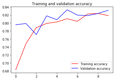
Fig. 5. Inception v3 Model Result
As you can see, using Inception v3 for transfer learning, we are able to obtain a validation accuracy of 0.8 after 10 epochs. This is a 14% improvement from the previous CNN model.
Remarks
In this simple example, we can see how transfer learning is able outperform a simple CNN model for the Fashion MNist dataset. In real-life, most of our images are often more difficult to classify. Therefore, being able to leverage on a pre-trained model is really a big step forward for the community!
You can check out this Jupyter notebook for the codes above.
Reference
[1] Laurence Moroney et al. Coursera: Convolutional Neural Networks in TensorFlow
[2] Christian Szegedy et al. Going Deeper with Convolutions
Thank you for reading! See you in the next post!