
Auto Arima with Pyramid
Time series forecasting is one of the common problems that we face everyday. Some of these include predicting equity prices, inventory levels, sales quantity, and the list goes on. In R, Auto ARIMA is one of the favourite time-series modelling techniques. However, if you are a Python user, you can implement that too using Pyramid. As Auto ARIMA has many tunable parameters, it is crucial for us to understand the mechanics behind this algorithm!
- What is Auto ARIMA?
- Autoregressive (AR)
- Moving Average (MA)
- ACF and PACF
- Autoregressive Moving Average (ARMA)
- Non-seasonal Autoregressive Integrated Moving Average (ARIMA)
- Seasonal Autoregressive Integrated Moving Average (ARIMA)
- Auto ARIMA with Pyramid
- Others
- Reference
What is Auto ARIMA?
At a high level, Auto ARIMA is a form of supervised learning for time series problems. Auto ARIMA is basically ARIMA with a gridsearch component, in order to find the best parameters based on metrics such as Akaike Information Criterion (AIC).
ARIMA stands for Autoregressive Integrated Moving Average. ARIMA can be further broken down into the Autoregressive (AR) part, the Moving Average (MA) part, and Integrated (I) part. AR and MA models can be used as independent models to generate time-series predictions. However, when combined together as an ARMA model, it can generate better predictions. The integrated component removes trends by using a differencing operator.
A non-seasonal ARIMA often defined along with three parameters p, d, and q, which are the parameters associated with the non-seasonal part of the model
A seasonal ARIMA takes in an additional four parameters P, D, Q, and m, which are the parameters associated with the seasonal part of the model.
Sounds like alot to take in isn’t it? Don’t worry, let’s go through the individual components one at a time!
✅ ARIMA consists of three main components:
1) Autoregressive
2) Integrated
3) Moving Average
Autoregressive (AR)
An AR(p) model can be defined as:
\[X_t = Z_t + \phi_1X_{t-1} + \dots + \phi_{p}X_{t-p}\]where,
- \(p\) is the number of orders of the AR model
- \(Z_t\) is a white noise term, and \(Z_t \sim iid(0, \sigma^2)\)
- \(X_t\) is the time-series numerical value at time \(t\)
- \(\phi_p\) is the parameter associated with the \(X_{t-p}\) term
Showing this in a spreadsheet might be easier to understand:
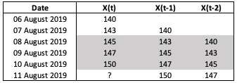
Fig. 1. AR Model Spreadsheet Example
Suppose we have 5 days worth of stock price. In order to obtain a AR(2) model, we fit a linear regression using \(X_{t_1}\) and \(X_{t_2}\) as independent variables and \(X_{t}\) as the dependent variable (see grey area of Figure 1). Note that, this assumes the both \(X_{t_1}\) and \(X_{t_2}\) are significant based on their respective p-values (i.e. less than 0.05). The parameters \(\phi\) are learnt using the linear regression.
Moving Average (MA)
A MA(q) model can be defined as:
\[X_t = \mu + Z_{t} + \theta_1 Z_{t-1} + \dots + \theta_q Z_{t-q}\]where,
- \(q\) is the number of orders of the MA model
- \(Z_t\) is a white noise error term, and \(Z_t \sim iid(0, \sigma^2)\)
- \(\theta_q\) is the parameter associated with the \(q^{th}\) \(Z\) term
Showing this in a spreadsheet might be easier to understand:
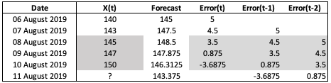
Fig. 2. MA Model Spreadsheet Example
MA model is more tedious compared to AR model. Let’s start by assuming we want to have a MA(2) model. The equation will look like \(X_t = \theta_0 Z_t + \theta_1 Z_{t-1} + \theta_2 Z_{t-2}\). In order to fit a linear regression on the error terms (see grey area of Figure 2), we will need to first generate the error terms. However, the error terms can only be generated when there is a forecast. Hence, we start at date \(\textit{06 August 2019}\) and forecast the price to be 145, the mean of the series. From there, we can compute the error term at date \(\textit{06 August 2019}\) as 5. On \(\textit{07 August 2019}\) we will have error term for \(t-1\) based on our previous calculation. We can then obtain the forecast for \(\textit{07 August 2019}\) by taking the mean and adjusting the forecast by its previous time period errors. Note that the parameters \(\theta\) are learnt using the linear regression, and I assume \(\theta_0\) to be 0.5 and \(\theta_1\) to be 0.25 in the example shown in Figure 2.
ACF and PACF
At this point, I will like to introduce Autocorrelation Function (ACF) and Partial Autocorrelation Function (PACF) as these two functions are ways to help us determine the number of orders for our AR model and MA model.
Autocorrelation Function
Autocorrelation function (ACF) is the Pearson Correlation Coefficient between the price at time \(t\) and the price at time \(t-k\), where \(k\) is the number of lag periods. The correlation between these two time periods represents both the direct and indirectly effects of previous period prices on the current period prices.
So for example, the correlation between \(X_t\) and \(X_{t-2}\) will contain the direct effect of \(X_{t-2}\) price on \(X_t\) and the indirect effect of \(X_{t-2}\) on \(X_t\), which came through \(X_{t-1}\). The intuition behind this is that prices two periods back could have a direct relationship with current day prices if there are systematic events that happen every two periods. At the same time, prices two periods back could influence prices one period back, which then influence current day prices. Thus the correlation betweeen \(X_t\) and \(X_{t-2}\) captures both these effects together, and we do not know if the effect is direct or indirect.
Let’s look at the computation via our spread sheet example:
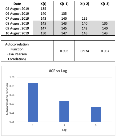
Fig. 3. Autocorrelation Function Spreadsheet Example
As seen in Figure 3, we calculate the correlation between \(X_t\) and \(X_{t-1}\) to obtain the ACF for lag period 1, \(X_t\) and \(X_{t-2}\) to obtain the ACF for lag period 2, so on and so forth. We can then plot the ACF against the lag periods to visualise the correlation between the prices of each lag period and the current day prices.
Partial Autocorrelation Function
Partial Autocorrelation Function (PACF) is the direct effect between two time period. This can be done by splitting the total effect into different time periods components, through the use of a linear regression.
To calculate the PACF of two lag period, we will need to use the following equation:
\[X_t = \phi_1X_{t-1} + \phi_2X_{t-2} + \epsilon_t\]\(\phi_2\) is the PACF for two lag period as it captures the direct effect between \(X_t\) and \(X_{t-2}\) while \(\phi_1\) captures the indirect effect between \(X_t\) and \(X_{t-2}\).
If I want to calculate the PACF of 3 lag period, we will need to extend the equation to:
\[X_t = \phi_1X_{t-1} + \phi_2X_{t-2} + + \phi_3X_{t-3} + \epsilon_t\]Now, \(\phi_3\) is the PACF for three lag period.
Let’s go back to our previous spreadsheet example to understand the computation:
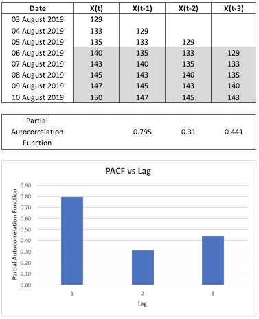
Fig. 4. Partial Autocorrelation Function Spreadsheet Example
Referring to Figure 4, in order to obtain PACF for one lag period, I fitted a linear regression of \(X_t\) against \(X_{t-1}\) - the coefficient of \(X_{t-1}\) is the PACF for one lag period. To obtain PACF for two lag periods, I fitted a linear regression of \(X_t\) against \(X_{t-1}\) and \(X_{t-2}\) - the coefficient of \(X_{t-2}\) is the PACF for two lag periods. Note that some of my variables were not statistically significant as the number of data points is very small.
Using PACF to obtain a better AR Model
For an AR Model, we only want to keep the lags where the direct magnitude of PACF are significant. We can identify these significant lag periods by looking at the periods where the PACF exceeds the confidence bands. This helps to ensure that we have a simpler model and avoid overfitting.
Going back to our example:
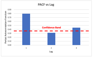
Fig. 5. Using PACF to Build a Better AR Model
Referring to Figure 5, suppose the confidence band is computed as \(\pm 0.35\), then a good AR model should contain only the first and third lag terms:
\[X_t = Z_t + \phi_1X_{t-1} + \phi_{3}X_{t-3}\]Note that the confidence band is defined as: \(\pm z_{1-{\alpha/2}} \sqrt{\frac{1}{n} \Bigl(1 + 2 \sum_{i=1}^k\rho(i)^2 \Bigl)}\)
Using ACF to obtain a better MA Model
As a general rule, a time series is well-modeled by a MA(q) model if ACF turns 0 when \(k\) (the lag period) > \(q\) (the order of the MA model). If that is not happening, then we will need to change \(q\).
Let’s go into more details on how I reached that conclusion.
Recall the equation of MA Model:
\[\begin{align} &\ X_t = \mu + Z_{t} + \theta_1 Z_{t-1} + \dots + \theta_q Z_{t-q} \\ &\ X_{t-k} = \mu+ + Z_{t-k} + \theta_1 Z_{t-k-1} + \dots + \theta_q Z_{t-k-q} \\ \end{align}\]Also, this is how ACF is calculated:
\[ACF = Correlation(X_t, X_{t-k}) = \frac{E[X_t X_{t-k}] - E[X_t]E[X_{t-k}]}{\sigma_t\sigma_{t-k}}\]where,
- k is the number of lag periods
When \(k\) (the lag period) > \(q\) (the order of the MA Model), there will be no identical error terms between \(X_t\) and \(X_{t-k}\). Any multiplication of two independent identical distributed error terms will be zero.
Therefore:
\[\begin{align} &\ ACF = \\ &\ \frac{E[X_t X_{t-k}] - E[X_t]E[X_{t-k}]}{\sigma_t\sigma_{t-k}} = \\ &\ \frac{E[\mu^2] - E[\mu]E[\mu]}{\sigma_t\sigma_{t-k}} = \\ &\ \frac{0}{\sigma_t\sigma_{t-k}} = 0\\ \end{align}\]When \(k\) (the lag period) \(<=\) \(q\) (the order of the MA Model), there will be identical error terms between \(X_t\) and \(X_{t-k}\). Multiplication of identical error terms will yield a non-zero expected value as \(E[Z_t^2] = Var(Z_t) + (E[Z_t])^2 > 0\), since \(Var(Z_t) > 0\).
Therefore:
\[\begin{align} &\ ACF = \\ &\ \frac{E[X_t X_{t-k}] - E[X_t]E[X_{t-k}]}{\sigma_t\sigma_{t-k}} = \\ &\ \frac{E[\mu^2 + x] - E[\mu]E[\mu]}{\sigma_t\sigma_{t-k}} \ne 0 \\ \end{align}\]where \(x\in\mathbb{R}\)
Autoregressive Moving Average (ARMA)
An ARMA(p, q) model is formed by simply combining AR(p) model and MA(q) model as follows:
\[X_t = Z_t + \phi_1X_{t-1} + \dots + \phi_{p}X_{t-p} + \mu+ \theta_1 Z_{t-1} + \theta_2 Z_{t-2} + \dots + \theta_q Z_{t-q}\]For current period prediction we will not have the current period error, hence:
\[\hat{X}_t = \phi_1X_{t-1} + \dots + \phi_{p}X_{t-p} + \mu+ \theta_1 Z_{t-1} + \theta_2 Z_{t-2} + \dots + \theta_q Z_{t-q}\]To decide on the order for the AR Model and MA Model, we would need to look at the ACF and PACF as explained previously.
Non-seasonal Autoregressive Integrated Moving Average (ARIMA)
AR, MA, and ARMA models requires the time series to be stationary, where stationary is defined as having a constant mean, constant variance overtime, and no seasonality.
When given a time series with a trend and no seasonality, the solution is to use a non-seasonal ARIMA model. It elimates the trend by applying differencing on the time series. This means that rather than predicting on the time series itself, we are going to predict the difference of the time series between one time stamp and another time stamp. The post-transformed time series is expected to be stationary. Usually it is sufficient to take the first order of differencing to eliminate the trend.
We can defined an ARIMA(p,1,q) model with first order of differencing as:
\[Y_t = Z_t + \phi_1Y_{t-1} + \dots + \phi_{p}Y_{t-p} + \mu+ \theta_1 Z_{t-1} + \theta_2 Z_{t-2} + \dots + \theta_q Z_{t-q}\]where,
- \(Y_t\) = \(X_t\) - \(X_{t-1}\)
Suppose we predicted \(Y_t\) and would like to obtain \(X_t\):
\[\begin{align} &\ X_t = \\ &\ Y_{t} + X_{t-1} = \\ &\ Y_{t} + Y_{t-1} + X_{t-2} = \\ &\ Y_{t} + Y_{t-1} + Y_{t-2} + X_{t-3} = \\ &\ \dots \\ &\ \sum_{i=0}^{t} Y_i + X_0 \end{align}\]As the equation of an ARIMA model is pretty long, the model is often simplified using backshift operators. A backshift operator creates a new variable which represents the the lagged terms. For example, when applied once, \(B(X_t) = X_{t-1}\). When applied twice, \(B^2(X_t) = X_{t-2}\). This allow us to create a more compact form of the equation that only involves backshifts operators and current values.
Let’s simplify the ARIMA model equation using backshift operators:
\[\begin{align} &\ Y_t = Z_t + \phi_1Y_{t-1} + \dots + \phi_{p}Y_{t-p} + \mu+ \theta_1 Z_{t-1} + \theta_2 Z_{t-2} + \dots + \theta_q Z_{t-q} \\ &\ Y_t - \phi_1Y_{t-1} - \dots - \phi_{p}Y_{t-p} = \mu + Z_t + \theta_1 Z_{t-1} + \theta_2 Z_{t-2} + \dots + \theta_q Z_{t-q} \\ &\ Y_t - \phi_1BY_{t} - \dots - \phi_{p}B^pY_{t} = \mu + Z_t + \theta_1BZ_{t} + \theta_2B^2Z_{t} + \dots + \theta_qB^qZ_{t} \\ &\ (1 - \phi_1B - \dots - \phi_{p}B^p)Y_t = \mu + (1 + \theta_1B + \theta_2B^2 + \dots + \theta_qB^q)Z_{t} \\ &\ (1 - \phi_1B - \dots - \phi_{p}B^p)(1-B)^dX_t = \mu + (1 + \theta_1B + \theta_2B^2 + \dots + \theta_qB^q)Z_{t} \\ \end{align}\]where,
- \(Y_t\) = \((1-B)^dX_t\), as \(Y_t\) is a differenced series that could be differenced more than once
Note: By multiplying a series by \((1-B)^d\), we are removing the trend of the time series. This concept will be used again in the next section when removing seasonality.
Seasonal Autoregressive Integrated Moving Average (ARIMA)
Seasonal Autoregressive Integrated Moving Average model should be used when the time series data contains seasonality and trends, where seasonality is a repeating pattern within a year.
On a high level, seasonal ARIMA model is defined as:
\[\text{ARIMA} (p,d,q)(P,D,Q)_m\]where,
- \((p,d,q)\) is the non-seasonal part of the model
- \((P,D,Q)\) is the seasonal part of the model
- \(m\) is the number of periods within a year for the seasonality to repeat
The seasonal terms are multiplied in to remove the seasonality. Recall in the previous section that such multiplication is used to remove trend and seasonality since we are basically creating a new series which is the difference bwtween two time periods.
For example, an \(\text{ARIMA}(1,d,1)(1,D,1)_m\) can be written as:
\[(1 - \phi_1B)(1-\Phi_1B^m)(1-B)^d(1-B^m)^DX_t = \mu + (1 + \theta_1B)(1+\Theta_1B^m)Z_{t}\]Auto ARIMA with Pyramid
If you have reach this point and understand most of it, then congratulations! All those concepts are definitely alot to take in! This section will focus on the implementation using Pyramid, which is in Python!
As you know, ARIMA has many parameters. So the term Auto ARIMA simply means running through a gridseach to find the best parameters for all the tunable parameters within an ARIMA model, based on metrics such as Akaike Information Criterion (AIC). Implementing it in Pyramid is as simple as stating the minimum and maximum bounds for each parameters.
Begin by cloning my blog repository:
git clone https://github.com/wngaw/blog.git
Now let’s install the relevant packages:
cd auto_arima_example/src
pip install -r requirements.txt
Import the relevant packages
import pandas as pd
from pyramid.arima import auto_arima
from statsmodels.tsa.seasonal import seasonal_decompose
In this problem, we are trying to predict United States industrial production index. The data set is US industrial production index. You can download it here.
# Import data
data = pd.read_csv("data/industrial_production.csv", index_col=0)

# Formatting
data.index = pd.to_datetime(data.index, format='%Y-%m-%d')
Visualizing the time series:
ax = data.plot()
fig = ax.get_figure()
fig.savefig("output/arima_raw_data_line_plot.png")
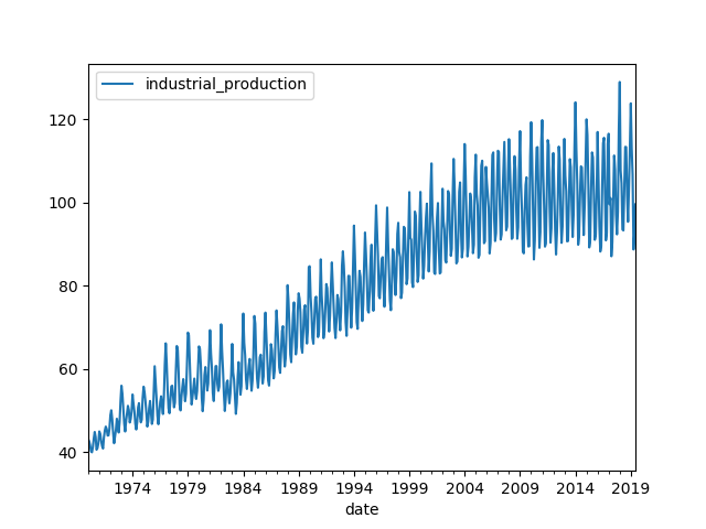
Fig. 6. Raw Data Line Plot
We can decomposed the time series to its trend component, seasonal component, and residual component:
result = seasonal_decompose(data, model='multiplicative')
fig = result.plot()
fig.savefig("output/seasonal_decompose_plot.png")
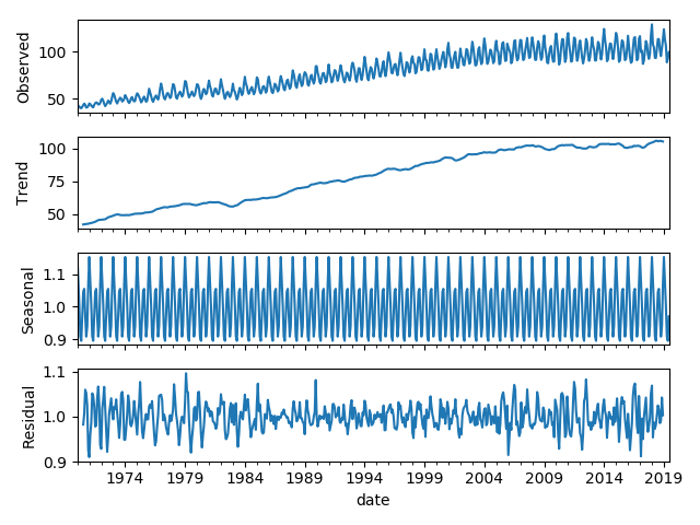
Fig. 7. Decomponsed Raw Data Line Plot
Finding best parameters for Seasonal ARIMA:
stepwise_model = auto_arima(data,
                            start_p=1, d=1, start_q=1,
                            max_p=3, max_d=1, max_q=3,
                            start_P=1, D=1, start_Q=1,
                            max_P=2, max_D=1, max_Q=2,
                            max_order=5, m=12,
                            seasonal=True, stationary=False,
                            information_criterion='aic',
                            alpha=0.05,
                            trace=True,
                            error_action='ignore',
                            suppress_warnings=True,
                            stepwise=True,
                            n_jobs=-1,
                            maxiter=10)

print(f'best_aic: {stepwise_model.aic()}')
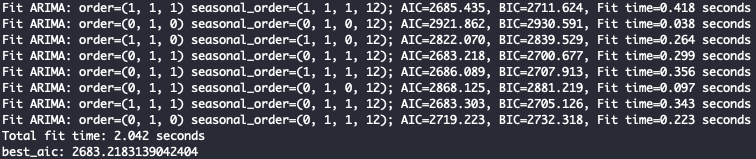
Fig. 8. Auto Arima Parameter Search Logs
Train test split and fit on train data:
# Train Test Split
train = data.loc['1985-01-01':'2016-12-01']
test = data.loc['2017-01-01':]

# Train
stepwise_model.fit(train)
Evaluate prediction result on test data:
future_forecast = stepwise_model.predict(n_periods=30)
future_forecast = pd.DataFrame(future_forecast, index=test.index, columns=['prediction'])
test_data_evaluation = pd.concat([test, future_forecast], axis=1)

ax = test_data_evaluation.plot()
fig = ax.get_figure()
fig.savefig("output/arima_evaluation_test_data_line_plot.png")
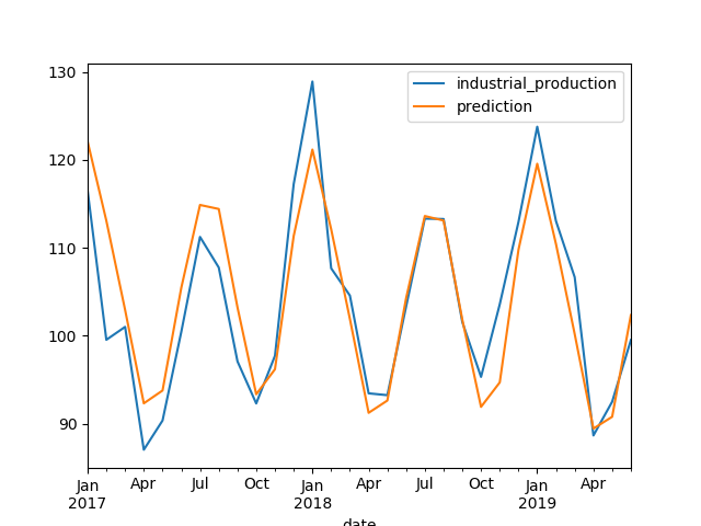
Fig. 9. Evaluation on Test Data
Overlaying test data predictions on full data set:
full_data_evaluation = pd.concat([data, future_forecast], axis=1)
ax = full_data_evaluation.plot()
fig = ax.get_figure()
fig.savefig("output/arima_evaluation_full_data_line_plot.png")
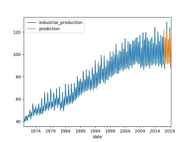
Fig. 10. Test Data Predictions overlay on Full Data
Others
In the content above, white noise is often included as a term. As such, I will like to go a little into the definition of white noise.
A white noise is a time series that meets three main conditions:
- Mean = 0
- Standard deviation is constant over time
- Correlation between lag period = 0
White noise is inherently not predictable.
Reference
[1] William Thistleton et al. Coursera: Practical Time Series Analysis
[2] Rob J Hyndman et al. OTexts: ARIMA models
[3] Jose Marcial Portilla Medium: Using Python and Auto ARIMA to Forecast Seasonal Time Series
Thank you for reading! See you in the next post!