
Sequence Modelling using CNN and LSTM
Sequence data is everywhere. One example is timestamped transactions, something that almost every company has. Increasingly companies are also collecting unstructured natural language data such as product reviews. While techniques like RNN are widely used for NLP problems, we can actually use it for any form of sequence-like predictions.Therefore, in this post I will explore more on how we can utilise CNN and LSTM for sequence modelling!
What is Sequence Modelling?
Sequence modelling is a technique where a neural network takes in a variable number of sequence data and output a variable number of predictions. The input is typically fed into a recurrent neural network (RNN).
There are four main variants of sequence models:
- one-to-one: one input, one output
- one-to-many: one input, variable outputs
- many-to-one: variable inputs, one output
- many-to-many: variable inputs, variable outputs
As most data science applications are able to use variable inputs, I will be focusing on many-to-one and many-to-many sequence models
⭐ As most data science applications are able to use variable number of inputs, I will be focusing on many-to-one and many-to-many sequence models
Quick recap on CNN and LSTM
Convolutional Neural Network (CNN) is a type of neural network architecture that is typically used for image recognition as the 2-D convolutional filters are able to detect edges of images and use that to generalise image patterns. In the case of sequence data, we can use a 1-D convolutional filters in order to extract high-level features.
Long-short Term Memory (LSTM) is a kind of recurrent neural network (RNN) that uses a special kind of cell that is able to memorise information by having gateways that pass through different cells. This is critical for long sequence data as a simple RNN without any special cells like LSTM or GRU suffers from the vanishing gradient problem.
Implementation
The following sections will be focusing on implementation using Python.
Dataset
The data set in the following example will be based on Sunspots dataset which is available at Kaggle by clicking here. Sunspots are temporary phenomena on the Sun’s photosphere that appear as spots darker than the surrounding areas. They are regions of reduced surface temperature caused by concentrations of magnetic field flux that inhibit convection. Sunspots usually appear in pairs of opposite magnetic polarity. Their number varies according to the approximately 11-year solar cycle.
Import libraries
Let’s start off by importing the necessary libraries.
import pandas as pd
import numpy as np
import matplotlib.pyplot as plt
import tensorflow as tf
from tensorflow.keras.utils import plot_model
Settings
split_time = 3000
window_size = 60  # Number of slices to create from the time series
batch_size = 32
shuffle_buffer_size = 1000
forecast_period = 30  # For splitting data in many-to-many sequence model
Helper functions
def plot_series(time, series, format="-", start=0, end=None):
    plt.plot(time[start:end], series[start:end], format)
    plt.xlabel("Time")
    plt.ylabel("Value")
    plt.grid(True)


def plot_loss(history):
    loss=history.history['loss']
    epochs=range(len(loss)) # Get number of epochs
    plt.plot(epochs, loss, 'r')
    plt.title('Training loss')
    plt.xlabel("Epochs")
    plt.ylabel("Loss")
    plt.legend(["Loss"])
Read data
df = pd.read_csv('data/Sunspots.csv', usecols=['Date', 'Monthly Mean Total Sunspot Number'])
Pre-processing
time = np.array(list(df.index))
sunspots = list(df['Monthly Mean Total Sunspot Number'])
series = np.array(sunspots)

time_train = time[:split_time]
train = series[:split_time]
time_test = time[split_time:]
test = series[split_time:]
Visualise time series
plt.figure(figsize=(10, 6))
plot_series(time, series)
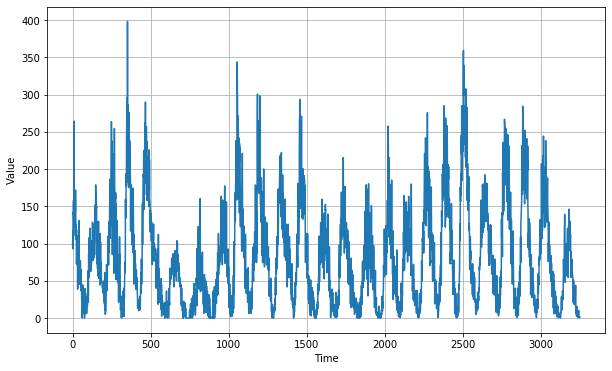
Fig. 1. Sunspots Time Series
Many-to-one sequence model
Pre-procesing
One of the distinctive step in sequence modelling is to convert the sequence data into multiple samples of predictor variables and target variable.
def windowed_dataset(series, window_size, batch_size, shuffle_buffer):
    """ Helper function that turns data into a window dataset"""
    series = tf.expand_dims(series, axis=-1)  # Expand dimensions
    ds = tf.data.Dataset.from_tensor_slices(series)
    ds = ds.window(window_size, shift=1, drop_remainder=True)  # Split a single time series to "window_size" slices with a time shift of 1, drops remainder of each slice to ensure uniform size across all slices.
    ds = ds.flat_map(lambda w: w.batch(window_size))
    ds = ds.map(lambda w: (w[:-1], w[-1:]))  # Data into features (x) and label (y)
    ds = ds.shuffle(shuffle_buffer)  # shuffle_buffer = number of data items
    ds = ds.batch(batch_size).prefetch(1)  # Batching the dataset into a groups of "batch_size"
    return ds
For inference, we just need to convert the data into multiple samples of predictor variables.
def model_forecast(model, series, window_size, batch_size):
    ds = tf.data.Dataset.from_tensor_slices(series)
    ds = ds.window(window_size, shift=1, drop_remainder=True)  # Split a single time series to "window_size" slices with a time shift of 1, drops remainder of each slice to ensure uniform size across all slices.
    ds = ds.flat_map(lambda w: w.batch(window_size))
    ds = ds.batch(batch_size).prefetch(1)
    forecast = model.predict(ds)
    return forecast
Defining model
For input, we are converting the time series into samples of 60 (window_size). The first 59 data points of a sample will be used as the predictor variables while the last data point will be used as the target variable.
tf.keras.backend.clear_session()
tf.random.set_seed(51)
np.random.seed(51)
train_set = windowed_dataset(train, window_size=window_size,
                             batch_size=batch_size, shuffle_buffer=shuffle_buffer_size)
model_many_to_one = tf.keras.models.Sequential([
  tf.keras.layers.Conv1D(filters=60, kernel_size=5,
                         strides=1, padding="causal",
                         activation="relu",
                         input_shape=[None, 1]),  # None = Model can take sequences of any length
  tf.keras.layers.LSTM(60, activation="tanh", return_sequences=True),
  tf.keras.layers.LSTM(60, activation="tanh", return_sequences=False),
  tf.keras.layers.Dense(30, activation="relu"),
  tf.keras.layers.Dense(10, activation="relu"),
  tf.keras.layers.Dense(1),
  tf.keras.layers.Lambda(lambda x: x * 100)  # LSTM's tanh activation returns between -1 and 1. Scaling output to same range of values helps learning.
])

# Note: to turn this into a classification task, just add a sigmoid function after the last Dense layer and remove Lambda layer.

optimizer = tf.keras.optimizers.SGD(lr=1e-5, momentum=0.9)
model_many_to_one.compile(loss=tf.keras.losses.Huber(), # Huber is less sensitive to outliers
                          optimizer=optimizer,
                          metrics=["mae"])
model_many_to_one.summary()
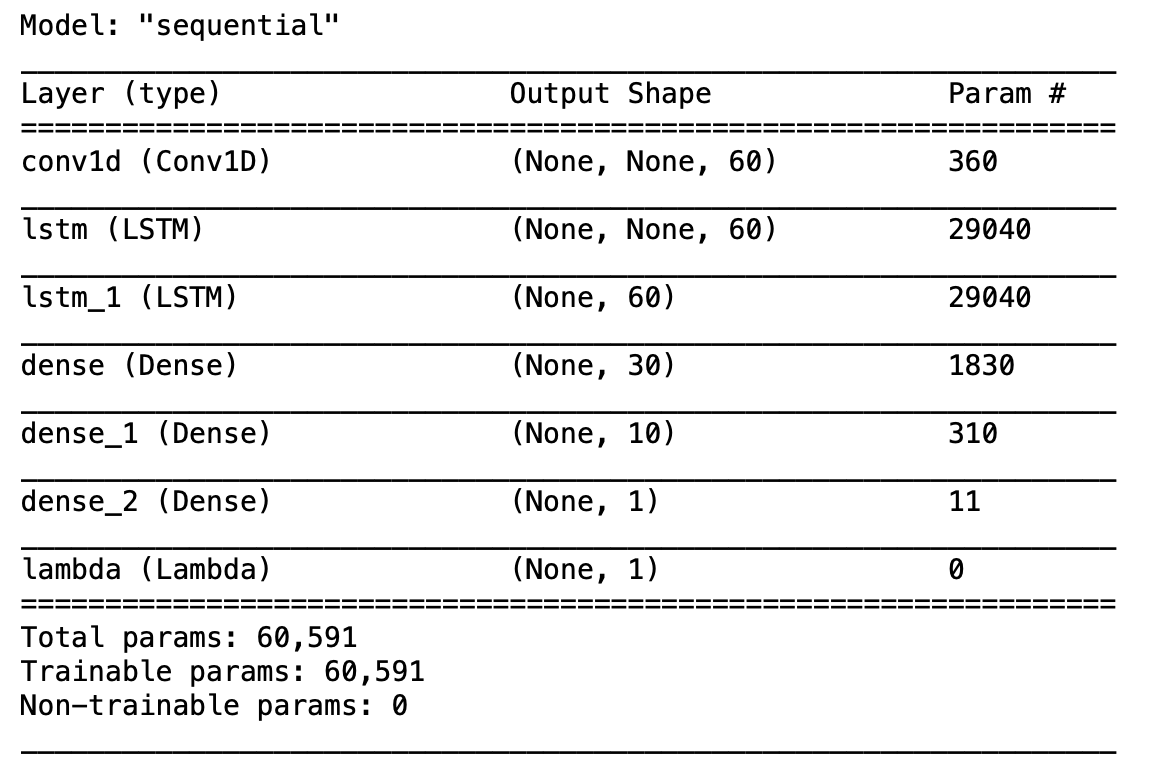
Fig. 2. Many-to-one Sequence Model Summary
Train
history = model_many_to_one.fit(train_set,epochs=10)
plot_loss(history)
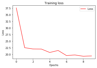
Fig. 3. Many-to-one Sequence Model Training Loss
Test
We will now use the trained model to predict values for the test set and evaluate it.
forecast = model_forecast(model_many_to_one,
                          series[..., np.newaxis],
                          window_size, batch_size)[split_time - window_size + 1:, 0]
MAE for test set is 10.82.
mae = tf.keras.metrics.mean_absolute_error(test, forecast).numpy()
Visualising predictions for the test set.
plt.figure(figsize=(10, 6))
plot_series(time_test, test)
plot_series(time_test, forecast)
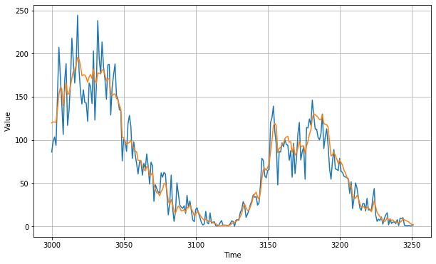
Fig. 4. Many-to-one Sequence Model Test Evaluation
Many-to-many sequence model
Pre-procesing
Similar to many-to-one, we need to convert the sequence data into multiple samples of predictor variables and target variable.
def windowed_dataset(series, window_size, batch_size, shuffle_buffer, forecast_period):
    """ Helper function that turns data into a window dataset"""
    series = tf.expand_dims(series, axis=-1)  # Expand dimensions
    ds = tf.data.Dataset.from_tensor_slices(series)
    ds = ds.window(window_size, shift=1, drop_remainder=True)  # Split a single time series to "window_size" slices with a time shift of 1, drops remainder of each slice to ensure uniform size across all slices.
    ds = ds.flat_map(lambda w: w.batch(window_size))
    ds = ds.map(lambda w: (w[:-forecast_period], w[forecast_period:]))  # Data into features (x) and label (y)
    ds = ds.shuffle(shuffle_buffer)  # shuffle_buffer = number of data items
    ds = ds.batch(batch_size).prefetch(1)  # Batching the dataset into a groups of "batch_size"
    return ds
Data conversion for inference data.
def model_forecast(model, series, window_size, batch_size):
    ds = tf.data.Dataset.from_tensor_slices(series)
    ds = ds.window(window_size, shift=1, drop_remainder=True)  # Split a single time series to "window_size" slices with a time shift of 1, drops remainder of each slice to ensure uniform size across all slices.
    ds = ds.flat_map(lambda w: w.batch(window_size))
    ds = ds.batch(batch_size).prefetch(1)
    forecast = model.predict(ds)
    return forecast
Defining model
For input, we are converting the time series into samples of 60 (window_size). The first 30 data points of a sample will be used as the predictor variables while the last 30 points will be used as the target variables.
tf.keras.backend.clear_session()
tf.random.set_seed(51)
np.random.seed(51)
train_set = windowed_dataset(train, window_size=window_size,
                             batch_size=batch_size, shuffle_buffer=shuffle_buffer_size,
                             forecast_period=forecast_period)
model_many_to_many = tf.keras.models.Sequential([
  tf.keras.layers.Conv1D(filters=60, kernel_size=5,
                         strides=1, padding="causal",
                         activation="relu",
                         input_shape=[None, 1]),  # None = Model can take sequences of any length
  tf.keras.layers.LSTM(60, activation="tanh", return_sequences=True),
  tf.keras.layers.LSTM(60, activation="tanh", return_sequences=True),
  tf.keras.layers.Dense(30, activation="relu"),
  tf.keras.layers.Dense(10, activation="relu"),
  tf.keras.layers.Dense(1),
  tf.keras.layers.Lambda(lambda x: x * 100)  # LSTM's tanh activation returns between -1 and 1. Scaling output to same range of values helps learning.
])

optimizer = tf.keras.optimizers.SGD(lr=1e-5, momentum=0.9)
model_many_to_many.compile(loss=tf.keras.losses.Huber(), # Huber is less sensitive to outliers
                           optimizer=optimizer,
                           metrics=["mae"])
model_many_to_many.summary()
Fig. 5. Many-to-many Sequence Model Summary
Train
history = model_many_to_many.fit(train_set,epochs=500)
plot_loss(history)
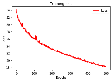
Fig. 6. Many-to-many Sequence Model Training Loss
Test
We will now use the trained model to predict values for the test set and evaluate it. Here we are splitting the test set in multiple chunks of 60 values, taking the first 30 values of each chunk as the predictors and the next 30 values as the targets.
# Using the past 30 values as inputs and predicting the next 30 values,
# iterate to get forecast for the entire test set

num_batch = 7
time_test_subset = np.array([])
test_subset = np.array([])
forecast_subset = np.array([])

for i in range(num_batch):
    if i == 0:
        time_test_chunk = time_test[-30:] # last 30 test timestep
        test_chunk = test[-30:] # last 30 test values
        series_chunk = test[-60:-30] # last 60 to last 30 as x values
        series_chunk = series_chunk.reshape(1, len(series_chunk), 1) # Reshape to 3D array for CNN
        forecast_chunk = model_many_to_many.predict(series_chunk).ravel()

        # Append chunks
        time_test_subset = np.append(time_test_chunk, time_test_subset)
        test_subset = np.append(test_chunk, test_subset)
        forecast_subset = np.append(forecast_chunk, forecast_subset)
    else:
        t1 = -30 * i
        t2 = -30 * (i + 1)
        t3 = -30 * (i + 2)
        time_test_chunk = time_test[t2:t1]
        test_chunk = test[t2:t1]
        series_chunk = test[t3:t2]
        series_chunk = series_chunk.reshape(1, len(series_chunk), 1) # Reshape to 3D array for CNN
        forecast_chunk = model_many_to_many.predict(series_chunk).ravel()

        # Append chunks
        time_test_subset = np.append(time_test_chunk, time_test_subset)
        test_subset = np.append(test_chunk, test_subset)
        forecast_subset = np.append(forecast_chunk, forecast_subset)
MAE for test set is 37.17, significantly higher than the many-to-one model. This indicates that many-to-many is a more difficult learning task compared to many-to-one. Further fine-tuning of model might be required. Firstly, we can try removing the trend and seasonality of the time series before fitting the model. Secondly, we can try increasing the window size to allow more inputs into the many-to-many sequence model. I will leave that for you to try it out!
mae = tf.keras.metrics.mean_absolute_error(test_subset, forecast_subset).numpy()
Visualising predictions for the test set.
plt.figure(figsize=(10, 6))
plot_series(time_test_subset, test_subset)
plot_series(time_test_subset, forecast_subset)
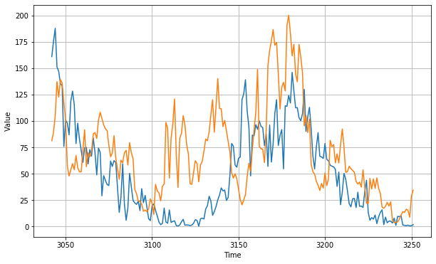
Fig. 7. Many-to-many Sequence Model Test Evaluation
Remarks
In this post, we have seen how we can use CNN and LSTM to build many-to-one and many-to-many sequence models. In real world applications, many-to-one can by used in place of typical classification or regression algorithms. On the other hand, many-to-many can be used when there is a need to predict a sequence of data such as the stock price for the next 6 months.
You can check out the Jupyter Notebook here.
Reference
[1] Laurence Moroney et al. Coursera: Sequences, Time Series and Prediction
[2] Jason Brownlee How to Develop 1D Convolutional Neural Network Models for Human Activity Recognition
Thank you for reading! See you in the next post!