
Statistical Power
Many time a company might have many features that it wants to roll out to its customers. However, no one really knows if a new feature is beneficial as it has never been implemented before. Hence, an experiment is usually set up to test its incremental benefit. A properly crafted experiment will allow the experimenter to understand what is the minimum sample size to collect before the experiment. During or after the experiment, the experimenter can also understand what is statistical power of the experiment and determine if he/she should collect more samples.
- Outcomes of a Hypothesis Test
- What is Statistical Power?
- Context
- Solving for: Effect Size, Statistical Power, and Sample Size
- Statistical Power with StatsModels
- Reference
Outcomes of a Hypothesis Test
Before we dive into statistical power, we need to recall the possible decision outcomes of a hypothesis test (see Figure 1). Type 1 Error is the probablity of rejecting \(H_0\) when \(H_0\) is true, denoted by \(\alpha\) (significance level). On the other hand, Type 2 Error is the probability of not rejecting \(H_0\) when \(H_a\) is true instead, denoted by \(\beta\).
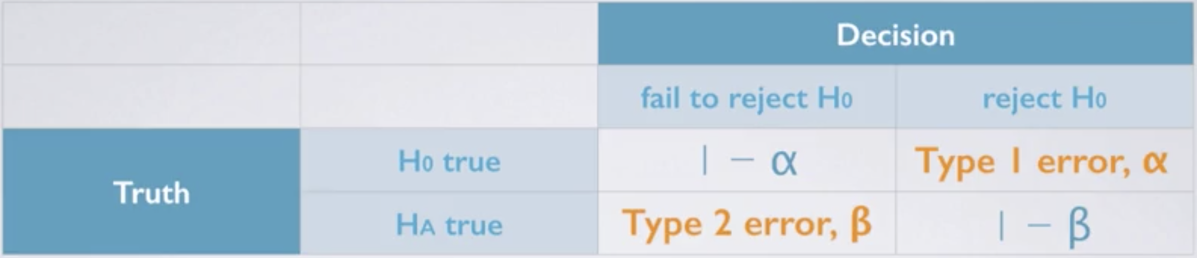
Fig. 1. Hypothesis Testing Outcomes - (Image source: here)
What is Statistical Power?
Statistical power is defined as the probability of correctly rejecting \(H_0\). In other words, it is defined as (1 - Type 2 error). In most experiments, a minimum of 80% statistical power is required to consider the test statistically significant. In a hypothesis test, our goal is to keep both \(\alpha\) and \(\beta\) low. Since \(\alpha\) and \(\beta\) are inversely related, the only way to reduce both simultaneously is to increase the sample size.
Context
Suppose, we invented a new drug that can reduce blood pressure. To test the effectivelness of the drug, we set up an experiment involving two groups of 100 users. The group that receives the treatment is the experimental group, the one that does not is the control group. The users have blood pressure that is normally distributed between 140 and 180 mmHg, with a standard deviation of 12 mmHg. We set the significance level \(\alpha\) at 5%.
\[s_{exp} = 12, s_{ctrl} = 12 \\ n_{exp}=100, n_{ctrl}=100 \\\]where
- \(s\) is the sample standard deviation
- \(n\) is the sample size
Setting Up the Hypothesis Test
We set up a two-tailed hypothesis test as we are interested in knowing if the drug would affect blood pressure both positively and negatively.
\[H_0: \mu_{exp} - \mu_{ctrl} = 0 \\ H_a: \mu_{exp} - \mu_{ctrl} \neq 0\]Calculating the Standard Error
Standard error is the measure of dispersion of sample means around the population mean. For difference in sample means, we can calculate the standarad error as follows:
\[SE_{(exp - ctrl)} = \sqrt{\frac{s_{exp}^2}{n_{exp}} + \frac{s_{ctrl}^2}{n_{ctrl}} } \\ = \sqrt{\frac{12^2}{100} + \frac{12^2}{100} } \\ = 1.70 mmHg\]Calculating the Margin of Error
\[\begin{align} &\ \text{Margin of Error} \\ &\ = Z_{0.025} * SE \\ &\ = invnorm(0.975) * SE \\ &\ = 1.96 * 1.70 \\ &\ = 3.332 \\ \end{align}\]Solving for: Effect Size, Statistical Power, and Sample Size
In such situation, we have three variables which depends on each other - Effect Size, Statistical Power, and Sample Size. At any point of time, only one can be solved while the other two need to be held constant.
Scenario 1: Solving for Effect Size
Since sample size \(n\) is large (>30), the distribution of the difference of the means is approximately normal by the Central Limit Theorem.
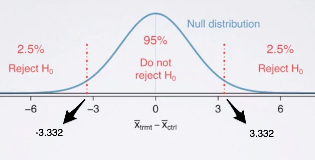
Fig. 2. Minimum Absolute Effect Size - (Image source: here)
With reference to the margin of error calculated previously, the minimum absolute effect size to reject \(H_0\) at 5% significance level is 3.332.
Scenario 2: Solving for Statistical Power
Suppose the observed effect size is -3 mmHg, that would mean that the observed distribution is to the left of the null distribution (see Figure 3).
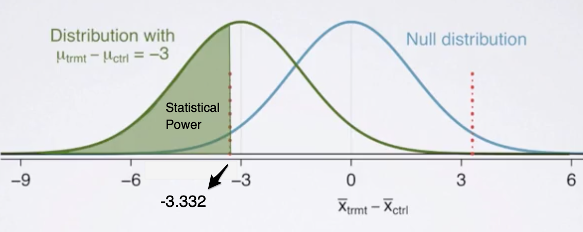
Fig. 3. Statistical Power - (Image source: here)
Since, statistical power is < 0.8, we consider the experiment not to be statistically significant.
Note: If the observed effect size is +3 mmHg instead, the observed distribution will be located at the right side of the null distribution, resulting in the same statistical power.
Scenario 3: Solving for Sample Size
Suppose the observed effect size is -3 mmHg, with a desired statistical power of 0.8.
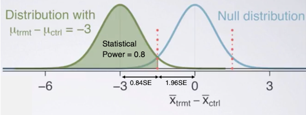
Fig. 4. Sample Size - (Image source: here)
Hence, the minimum sample size is 251 users in order to achieve a stastical power of 80%, assuming an effect size of -3 mmHg.
Statistical Power with StatsModels
Solving these parameters is rather straight forward and can be implemented using StatsModels. Note that I implemented a two-tailed z-test which assumes that the sample size \(n\) is large (> 30). If sample size \(n\) is small (<= 30), you will need to implement a t-test instead. Just replace NormalIndPower with TTestIndPower within the source code.
Begin by cloning my blog repository:
git clone https://github.com/wngaw/blog.git
Now let’s install the relevant packages:
cd statistical_power_example/src
pip install -r requirements.txt
To solve for statistical power:
from stats_power_solver import solve_statistical_power_z_test
statistical_power = solve_statistical_power_z_test(mean_exp=50, mean_ctrl=40, sd_exp=4, sd_ctrl=3, num_exp=200, num_ctrl=40, alpha=0.05)
print("statistical power: %0.3f" % (statistical_power))
You should see this:
\[\text{statistical power: 1.000}\]To solve for minimum sample size:
from stats_power_solver import solve_sample_size_z_test
num_exp, num_ctrl = solve_sample_size_z_test(abs_effect_size=0.1, ctrl_exp_ratio=0.2, statistical_power=0.8, alpha=0.05)
print("minimum sample size for experimental group: %0.f" % (num_exp))
print("minimum sample size for control group: %0.f" % (num_ctrl))
You should see this:
\[\begin{align} &\ \text{minimum sample size for experimental group: 4709} \\ &\ \text{minimum sample size for control group: 942} \\ \end{align}\]To solve for absolute effect size:
from stats_power_solver import solve_abs_effect_size_z_test
abs_effect_size = solve_abs_effect_size_z_test(num_exp=200, num_ctrl=40, statistical_power=0.8, alpha=0.05)
print("required abs_effect_size to reject H0: %0.3f" % (abs_effect_size))
You should see this:
\[\text{required abs_effect_size to reject H0: 0.485}\]Reference
[1] Mine Çetinkaya-Rundel Coursera: Inferential Statistics
Thank you for reading! See you in the next post!