
Decision Trees
Decision tree is one of the most interpretable machine learning model. However, it tends to overfit when learning the decision boundaries of the training data. Hence, decision trees are usually used as the base learner of ensembling methods such as Gradient Boosting and Random Forest. These ensemnbling methods have seen extreme success in the data science world. XGBoost, LightGBM, and Catboost are some of the popular gradient boosting methods that are widely used in competitions. But before getting there, we need to first understand how decision tree works as the base learner.
- What is Decision Tree?
- Hypothesis
- Context
- An Intuitive Explanation
- Types of Decision Trees
- Decision Tree Learning Algorithms
- Metrics
- Reference
What is Decision Tree?
Decision tree is a supervised learning algorithm that is capable of learning non-linear hypothesis through series of if-else statements. Compared to linear regressions and neural networks, decision tree is a much simpler learning algorithm. Decision tree can be used for both regression and classification problems.
✅ Decision trees are used as a base learner for more complicated algorithms such as Random Forest and Gradient Boosted Machine.
Hypothesis
The hypothesis of a decision tree is represented by a series of if-else statements that outputs the probability of a class for classification and a numerical value for regression.
Context
Assume we have the following dataset where we want to predict a fruit label given the color and diameter of it:
| Dataset | Color | Diameter | Label |
|---|---|---|---|
| TRAIN | GREEN | 3 | APPLE |
| TRAIN | YELLOW | 3 | APPLE |
| TRAIN | RED | 1 | GRAPE |
| TRAIN | RED | 1 | GRAPE |
| TRAIN | YELLOW | 3 | LEMON |
An Intuitive Explanation
The learning algorithm starts with the root node where it will receive the entire training set. Since CART is used as the learning algorithm for a classifcation problem, gini impurity is the metric we calculate.
The algorithm will start by calculating the gini impurity at the root node, which turns out to be 0.64. Then it will iterate over every value to create multiple true-false question where we can partition the data.
Possible questions are:
- Is the diameter >= 3?
- Is the diameter >=1?
- Is the color green?
- Is the color yellow?
- Is the color red?
At each iteration, gini impurity will be calculated for both child nodes. A weighted average gini impurity will be calculated based on the number of data points in each child nodes. This is because we care more about the gini impurity of a child node with more data points.
The information gain is then calculated by taking the difference between the gini impurity at the root node and the weighted average gini impurity at the child nodes. The best question is the one with the highest information gain.
For example, using the question \(\textit{Is the color green}\), the weighted average gini impurity of the child nodes is \(\mathbf{0.5}\) \(((\frac{4}{5} * 0.62) + (\frac{1}{5} * 0))\), giving us an information gain of \(\mathbf{0.14}\) \((0.64 - 0.5)\).
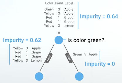
Fig. 1. Is Color Green? - (Image source: here)
The information gain is then calculated for every question:
| Question | Information Gain |
|---|---|
| Diameter >= 3? | 0.37 |
| Diameter >=1? | 0 |
| Color == Green? | 0.14 |
| Color == Yellow? | 0.17 |
| Color == Red? | 0.37 |
Here we can see that there is a tie between \(\textit{Is diameter >= 3?}\) and \(\textit{Is the color red?}\). Hence, we will choose the first question to be the best one. We then split the root node using this question.
Next, we will then repeat the process of splitting on the \(\textit{true}\) branch. Here, we found out that \(\textit{Is color yellow?}\) is the best question at this child node. We then split the child node using this question.
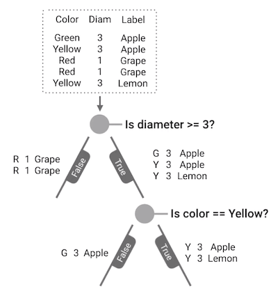
Fig. 1. Is Color Yellow? - (Image source: here)
Continuing the process, we found out that the information gain is 0 since there is no more question to be asked as both data points on the \(\textit{true}\) branch have identical color and diameter features. Hence, this node becomes a leaf node which predicts Apple at 50% and Lemon at 50%.
Since the node at the end of the \(\textit{true}\) branch has turned into a leaf node, we will then go over to the false branch to continue splitting. Over here, we found out that there is also no information gain since there is only one data point. Hence, this turns into a leaf node as well. At this point, \(\text{Is the color yellow?}\) becomes a decision node as it is where a decision has to be made.
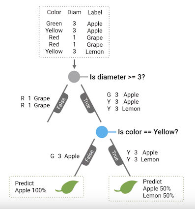
Fig. 1. Is Color Yellow? Leaf Nodes - (Image source: here)
Now, we return to the root node to split for the false branch. Similarly, we realise that there are no further questions to be asked that can give us information gain. Hence, this turns into a leaf node as well. At this point, \(\text{Is the diameter >= 3?}\) becomes a decision node as well, and the decision tree is fully built.
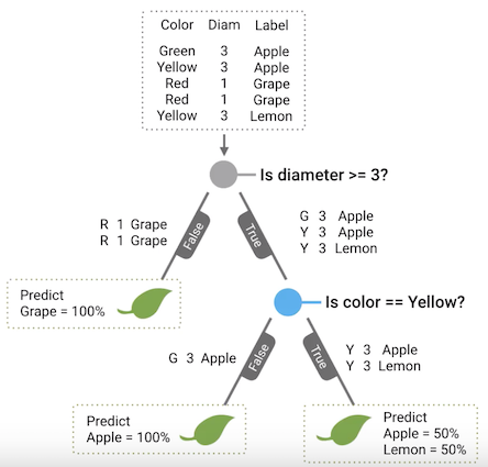
Fig. 1. Is Diameter >= 3? - (Image source: here)
Although the entire process seems complicated, it can actually be represented by a concise block of code as follows:
def build_tree(rows):
    gain, question = find_best_split(rows)
    if gain == 0:
        return Leaf(rows)
    true_rows, false_rows = partition(rows, question)
    true_branch = build_tree(true_rows)
    false_branch = build_tree(false_rows)
    return Decision_Node(question, true_branch, false_branch)
Types of Decision Trees
There are mainly two kinds of decision trees - classification tree and regression tree. In a classification tree, the predicted class is obtained by selecting the class with the highest probability at the leaf node where if-else criteria are met. In a regression tree, the predicted value is the average response of observations falling in that leaf node.
Decision Tree Learning Algorithms
Under the hood, the series of if-else statements of a decision tree can be generated using several kinds of learning algorithms:
Metrics
For decision trees, different algorithms use different metrics to decide on the best split points. Within each algorithm, classification and regression use different metrics as well. For classification, entropy and gini impurity are common metrics to evaluate at each split points when generating a decision tree. On the other hand, for regression, variance is usually used instead.
Entropy - For Classification
This metric measures the amount of disorder in a data set with a lowest value of 0, where a lower value is better as it indicates less uncertainty at a node. In laymen terms, it is how surprising a randomly selected item from the set is. If the entire data set were As, you will never be surprised to see an A, so entropy is 0.
The formula is as follows:
\[H(X) = \sum\limits_{i=1}^n p(x_i)log_2(\frac{1}{p(x_i)} )\]Gini Impurity - For Classification
This metric ranges between 0 and 1, where a lower value is better as it indicates less uncertainty at a node. It represents the probability of being incorrect if you randomly pick an item and guess its label.
The formula is as follows:
\[I_G(i) = 1 - \sum\limits_{j=1}^m f(i,j)^2\]Variance - For Regression
This metric measures how much a list of numbers varies from the average value, where a lower value is better as it indicates less uncertainty at a node. It is calculated by averaging the squared difference of every number from the mean.
The formula is as follows:
\[\sigma^2 = \frac{1}{N} \sum\limits_{i=1}^N (x_i - \bar{x})^2\]Reference
[1] Josh Gordon Machine Learning Recipes #8
[2] Toby Segaram Programming Collective Intelligence
Thank you for reading! See you in the next post!