
Neural Networks
The field of artificial intelligence (AI) was founded in 1956. For the next 56 years till 2012, artificial intelligence was not widely adopted due to reasons such as lack of computing power, fundings, among others. In 2012, the one and only AI breakthrough happened and many AI applications started to build on top of this discovery.
So what happened?
In 2012, two parallel ideas coincides during an AI competition called ImageNet, which is an object detection challenge that consists of 150,000 images across 1,000 object categories. This repository was collected by Princeton professor Fei-Fei Li across several year, who believes that showing learning algorithm more data was more important that creating the perfect learning algorithm. At the same time, a team from the University of Toronto uses Li’s massive amount of data to learn a neural network, which was an idea that took inspiration from how the brain learns.
The Toronto team entered the ImageNet challenge with their trained neural network and became the first team to break 75% accuracy in the competition. Neural network was then used year after year by every subsequent winning teams.
- What is Neural Network?
- Hypothesis
- Cost Function
- Gradient Descent
- Forward Propagation
- Back Propagation
- Reference
What is Neural Network?
Neural networks is a supervised learning algorithm that is capable of learning non-linear hypothesis.
✅ It is very important to understand the basic mechanics such as cost function, gradient descent, forward and backward propagation as all neural networks are built based on these concepts.
Hypothesis
A neural networks consists of an input layer, hidden layer(s), and an output layer. Within each hidden layer and output layer, there can be several neurons. Each neuron takes in inputs, weights, and biases from the previous layer, before passing it through an activation function to obtain an output value.
Visually, it looks as follow:
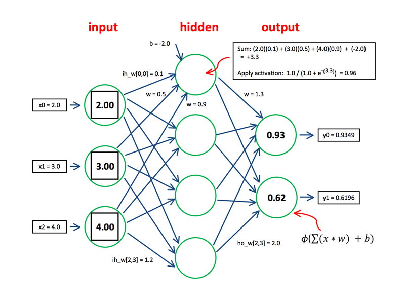
Fig. 1. Multi-Layer Perceptron Neural Network - (Image source: here)
The hypothesis of a multi-layer perceptron neural networks with a single node at the final layer is represented by the following function:
\[\begin{align} &\ a_1^{j-1} = g(\Theta_{1,0}^{(j-2)}x_0 + \Theta_{1,1}^{(j-2)}x_1 + ... + \Theta_{1,n}^{(j-2)}x_n) \\ &\ a_2^{j-1} = g(\Theta_{2,0}^{(j-2)}x_0 + \Theta_{2,1}^{(j-2)}x_1 + ... + \Theta_{2,n}^{(j-2)}x_n) \\ &\ ... \\ &\ a_i^{j-1} = g(\Theta_{i,0}^{(j-2)}x_0 + \Theta_{i,1}^{(j-2)}x_1 + ... + \Theta_{i,n}^{(j-2)}x_n) \\ \\ &\ h_{\Theta}(x) = a_{1}^{j} = g(\Theta_{1,0}^{(j-1)}a_{0}^{(j-1)} + \Theta_{1,1}^{(j-1)}a_{1}^{(j-1)} + ... + \Theta_{1,i}^{(j-1)}a_{i}^{(j-1)}\\ \end{align}\]where
- \(j\) is the total number of layers, which includes input and output layer
- \(i\) is the number of neurons in the \(j-1\) layer
- \(n\) is the number of input neurons in the \(j-2\) layer
- \(g(x)\) is the activation function that takes in the inputs and weights
- \(a_1^{j-1}\) represents the \(i^{th}\) neuron in layer \(j\)
- \(\Theta^{(j)}\) represents the matrix of weights controlling function mapping from layer \(j\) to \(j+1\)
Cost Function
Recall that the cost function for a regularized logistic regression is:
\[\begin{align} &\ J(\theta) = \frac{1}{m} \Biggl[ \sum\limits_{i=1}^m (h_\theta(x^i) - y^i)^2 + \lambda \sum\limits_{j=1}^n \theta_j^2 \Biggl] \end{align}\]The cost function for neural networks is an extended version of that:
\[\begin{align} &\ J(\theta) = \frac{1}{m} \Biggl[ \sum\limits_{i=1}^m \sum\limits_{k=1}^K ((h_\theta(x^i))_{k} - y_{k}^i)^2 + \lambda \sum\limits_{l=1}^{L-1} \sum\limits_{a=1}^{s_{l}} \sum\limits_{b=1}^{s_{l+1}} (\Theta_{b, a}^{l})^2 \Biggl] \end{align}\]where
- \(i\) is one of the \(m^{th}\) training samples
- \(k\) is one of the \(K\) output nodes
- \(l\) is one of the \(L-1\) layers, which excludes the output layer
- \(L\) is the total number of layers in the network, including the input and output layers
- \(s_{l}\) is the number of nodes (not counting bias node) in layer \(l\)
- \(a\) is one of the \(s_{l}\) nodes in layer \(l\)
- \(b\) is one of the \(s_{l+1}\) nodes in layer \(l+1\)
In the first part of the equation, the nested summations of the error term is added to account for multiple output nodes for multiclass classification. In the second part of the equation, the nested summation is added to account for every parameters in the entire network.
Similar to logistic regression, the overall objective is to minimise the cost function.
\[\begin{align} \underset{\theta_0,\ \ldots,\ \theta_n}{\min} J(\theta_0,\ \ldots,\ \theta_n) \end{align}\]Gradient Descent
Similar to linear and logistic regression, the gradient descent algorithm is used to update the values of the parameters:
\[\begin{align} \text{repeat until convergence} \ \left \{ \Theta_{ab}^{l} := \Theta_{ab}^{l} - \alpha \frac{\partial}{\partial \Theta_{ab}^{l}} J(\Theta) \right \}\\ \end{align}\]where
- \(a\) is one of the \(s_{l}\) nodes in layer \(l\)
- \(b\) is one of the \(s_{l+1}\) nodes in layer \(l+1\)
- \(l\) is one of the \(L-1\) layers, which excludes the output layer = \(\Theta\) is a vector of all the parameters (aka weights) within the neural network
- \(\alpha\) is the learning rate
Note: The notation for the parameters is changed slightly in order to identify the parameters’ position within the neural network.
However, in order to calculate the partial derivative term \(\frac{\partial}{\partial \Theta_{ab}^{l}} J(\Theta)\), we first need to compute the cost function \(J(\Theta)\) using forward propagation, then backpropagate the error terms for each node within the hidden layers, in order to finally compute the gradients required for the parameters update within gradient descent.
Forward Propagation
Forward propagation refers to the prediction of a training sample by passing the inputs values through a neural network.
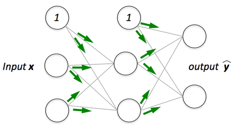
Fig. 2. Forward Propagation - (Image source: here)
Within the neural network, each neuron (excluding those in the input layer) first calculates the weighted sum of inputs \(Z_{a}^{l}\), before passing the \(Z_{a}^{l}\) into an activation function in order to obtain the activation value \(A_{a}^{l}\), where \(a\) is one of the neurons in layer \(l\) (see figure 3).
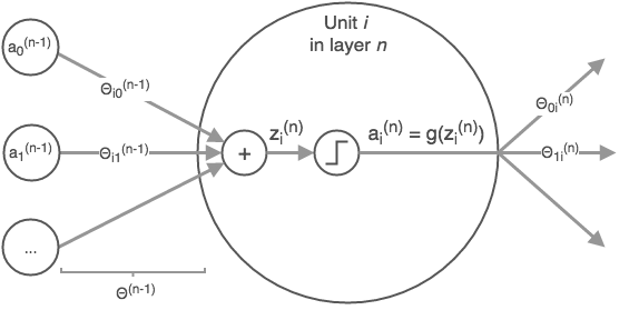
Fig. 3. Forward Propagation Calculation - (Image source: here)
Mathematically, the prediction values are calculated iteratively through each layer via the following:
\[\begin{align} &\ Z^2 = \Theta^1A^1 \\ &\ A^2 = g(Z^2) \\ &\ \ldots \\ &\ Z^{L} = \Theta^{L-1}A^{L-1} \\ &\ A^L = g(Z^L)\\ &\ h_\Theta(x) = A^L \end{align}\]where
- \(A^{L-1}\) is a vector of input values which include the bias value in the previous layer
- \(\Theta^{L-1}\) is a vector of parameters that connects the layer \(L-1\) and layer \(L\)
- \(Z^L\) is a vector consisting the weighted sum of inputs for each node in layer \(L\)
- \(g(x)\) is an activation function
- \(h_\Theta(x)\) is the output of the hypothesis which is also the activation value of the final layer
- \(L\) is the total number of layers in the neural network
Back Propagation
After obtaining the prediction values through forward propagation, we then calculate the error terms of the output layer and backpropagate this error terms backwards untill the second layer of the neural network. Backpropagation simply means the calculation of errors for each node in each of the previous layers.
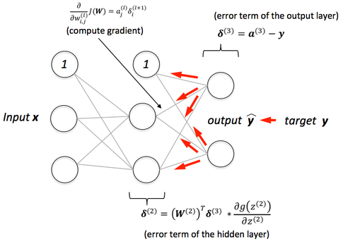
Fig. 4. Back Propagation - (Image source: here)
Mathematically, the calculation of the error terms for backpropagation is as follows:
\[\begin{align} &\ \delta^L = A^L - y \\ &\ \delta^{L-1} = (\Theta^{L-1})^T \delta^L * \frac{\partial (g(Z^{L-1}))}{\partial (Z^{L-1})} \\ &\ \delta^{L-2} = (\Theta^{L-2})^T \delta^{L-1} * \frac{\partial (g(Z^{L-2}))}{\partial (Z^{L-2})} \\ &\ \cdots \\ &\ \delta^{2} = (\Theta^{2})^T \delta^{3} * \frac{\partial (g(Z^{2}))}{\partial (Z^{2})} \\ \end{align}\]where
- \(\delta^L\) is a vector of error terms in layer \(L\)
- \(A^L\) is a vector of activation value in layer \(L\)
- \(y\) is a vector of actual target value with respect to each output nodes in the output layer \(L\)
- \(L\) is the total number of layers in the neural network
- \(\Theta^{L-1}\) is a vector of parameters that connects the layer \(L-1\) and layer \(L\)
- \(g(x)\) is an activation function
- \(Z^{L-1}\) is a vector consisting the weighted sum of inputs for each node in layer \(L-1\)
Once the error terms have been computed, we can then compute the gradients using the following derived formula (assuming the regularisation parameter \(\lambda\) = 0):
\[\begin{align} \frac{\partial }{\partial (\Theta_{ab}^l)} J(\Theta) = A_a^{l} \delta_b^{(l+1)} \end{align}\]where
- \(a\) is one of the nodes in layer \(l\)
- \(b\) is one of the nodes in layer \(l+1\)
- \(\Theta_{ab}^{l}\) is the parameter that connects node \(a\) in layer \(l\) and node \(b\) in layer \(l+1\)
Now that we have the gradients for each parameters, we can finally update the parameter using gradient descent. This entire process is then repeated several times by iterating through the entire dataset again in order to update the parameters to the point where the cost function is minimised.
Reference
[1] Andrew Ng Coursera: Machine Learning
Thank you for reading! See you in the next post!