
Logistic Regression
Logistic regression is one of most widely used classification learning algorithms in various fields, including machine learning, most medical fields, and social sciences. Similar to the post on linear regression, I will go into the mechanics behind logistic regression in order for us to gain a deeper understanding of it.
- What is logistic regression?
- Hypothesis
- Cost function
- Gradient Descent
- Advanced Optimization Algorithms
- Multiclass Classification
- Bias-Variance Tradeoff
- Regularization
- Logistic Regression with Scikit-Learn
- Reference
What is logistic regression?
Logistic regression is a supervised learning algorithm that outputs values between zero and one.
✅ Even logistic regression is one of the simplest binary classifier, it is actually one of the most adopted!
Hypothesis
The objective of a logistic regression is to learn a function that outputs the probability that the dependent variable is one for each training sample.
To achieve that, a sigmoid / logistic function is required for the transformation.
A sigmoid function is as follows:
\[\begin{align} f(x) = \frac{1}{1 + e^{-x}} \end{align}\]Visually, it looks like this:
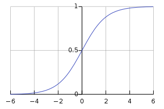
Fig. 1. Sigmoid Function - (Image source: here)
This hypothesis is typically represented by the following function:
\[\begin{align} &\text{h}_\theta(x) = \frac{1}{1+e^{-\theta^Tx}} \end{align}\]where
- \(\theta\) is a vector of parameters that corresponds to each independent variable
- \(x\) is a vector of independent variables
Cost function
The cost function for logistic regression is derived from statistics using the principle of maximum likelyhood estimation, which allows efficient identification of parameters. In addition the covex property of the cost function allow gradient descent to work effectively.
\[\begin{align} &\ J(\theta) = \frac{1}{m} \sum\limits_{i=1}^m (h_\theta(x^i) - y^i)^2 \\ &\ (h_\theta(x^i) - y^i)^2 = \left \{ \begin{array}{l} &\ -log(h_\theta(x^i)) \ \text{if} \ y^i = 1\\ &\ -log(1 - h_\theta(x^i)) \ \text{if} \ y^i = 0 \end{array} \right . \end{align}\]where
- \(i\) is one of the \(m^{th}\) training samples
- \(h_\theta(x^i)\) is the predicted value for the training sample \(i\)
- \(y^i\) is the actual value for the training sample \(i\)
To understand the cost function, we can look into each of the two components in isolation:
Suppose \(y^i = 1\):
- if \(h_\theta(x^i) = 1\), then the prediction error = 0
- if \(h_\theta(x^i) = 0\), then the prediction error approaches infinity
These two scenarios are represented by the blue line in Figure 2 below.
Suppose \(y^i = 0\):
- if \(h_\theta(x^i) = 0\), then the prediction error = 0
- if \(h_\theta(x^i) = 1\), then the prediction error approaches infinity
These two scenarios are represented by the red line in Figure 2 below.
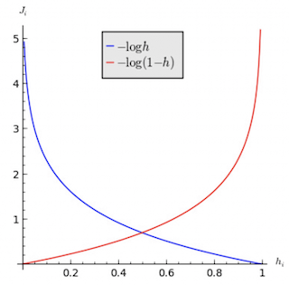
Fig. 2. Logistic Regression Cost Function - (Image source: here)
The logistic regression cost function can be further simplified into a one line equation:
\[\begin{align} &\ J(\theta) = \frac{1}{m} \sum\limits_{i=1}^m (h_\theta(x^i) - y^i)^2 \\ &\ (h_\theta(x^i) - y^i)^2 = -y^i log(h_\theta(x^i)) - (1-y^i)log(1- h_\theta(x^i) \end{align}\]The overall objective is to minimise the cost function by iterating through different values of \(\theta\).
\[\begin{align} \underset{\theta_0,\ \ldots,\ \theta_n}{\min} J(\theta_0,\ \ldots,\ \theta_n) \end{align}\]Gradient Descent
The gradient descent algorithm is as follows:
\[\begin{align} \text{repeat until convergence} \ \left \{ \theta_j := \theta_j - \alpha \frac{\partial}{\partial \theta_j} J(\theta_0,\ \ldots,\ \theta_n) \right \}\\ \end{align}\]where
- values of \(j = 0, 1,\ \ldots,\ n\)
- \(\alpha\) is the learning rate
Note: The gradient descent algorithm is identical to linear regression’s.
Advanced Optimization Algorithms
However, gradient descent is not the only algorithm that can minimize the cost function. Other advanced optimization algorithms are:
- Conjugate gradient
- BFGS
- L-BFGS
While these advanced algorithms are more complex and difficult to understand, they have the advantages of converging faster and not needing to pick learning rate \(\alpha\).
Multiclass Classification
One-vs-rest is a method where you turn a n-class classification problem into a nth seperate binary classification problem.
To deal with a multiclass problem, we then train a logistic regression binary classifier \(h_\theta^i (x)\) for each class \(i\) to predict the probability that y = i.
The prediction output for a given new input \(x\) will be chosen based on the classifier that has the highest probability.
\[\underset{i}{\min} h_\theta^i (x)\]where
- \(h_\theta^i (x)\) is the \(i^{th}\) binary classifier
Bias-Variance Tradeoff
Overfitting occurs when the algorithm tries too hard to fit the training data. This usually results in a learned hypothesis that is too complex, fails to generalize to new examples, and a cost function that is very close to zero on the training set.
On the contrary, underfitting occurs when the algorithm tries too little to fit the training data. This usually results in a learned hypothesis that is not complex enough, and fails to generalize to new examples.
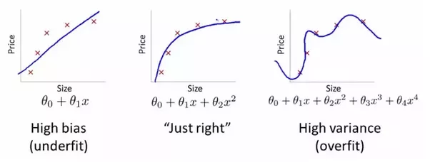
Fig. 3. Underfitting and Overfitting - (Image source: here)
Conceptually speaking, bias measures the difference between model predictions and the correct values. Variance refers to the variability of a model prediction for a given data point if you re-build the model multiple times.
As seen in Figure 4, the optimal level of model complexity is where prediction error on unseen data points is minimized. Below the optimal level of model complexity, bias will increase while variance will decrease due to a hypothesis that is too simplified. On the contrary, a very complex model will result in a low bias and high variance situation.
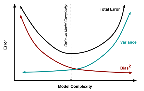
Fig. 4. Bias-Variance Tradeoff - (Image source: here)
Regularization
For a model to generalize well, regularization is usually introduced to reduce overfitting of the training data.
This is represented by a regularization term, \(\lambda \sum\limits_{j=1}^n \theta_j^2\), that is added to the cost function that penalizes all parameters \(\theta_1 \ldots,\ \theta_n\) that are high in value. This leads to a simpler hypothesis that is less prone to overfitting.
The new cost function then becomes:
\[\begin{align} &\ J(\theta) = \frac{1}{m} \Biggl[ \sum\limits_{i=1}^m (h_\theta(x^i) - y^i)^2 + \lambda \sum\limits_{j=1}^n \theta_j^2 \Biggl] \end{align}\]where
- \(i\) is one of the \(m^{th}\) training samples
- \(h_\theta(x^i)\) is the predicted value for the training sample \(i\)
- \(y^i\) is the actual value for the training sample \(i\)
- \(\lambda\) is the regularization parameter that controls the tradeoff between fitting the training dataset well and having the parameters \(\theta\) small in values
- \(j\) is one of the \(n^{th}\) parameters \(\theta\)
Overall objective remains the same:
\[\begin{align} \underset{\theta_0,\ \ldots,\ \theta_n}{\min} J(\theta_0,\ \ldots,\ \theta_n) \end{align}\]Gradient descent remains the same as well:
\[\begin{align} \text{repeat until convergence} \ \left \{ \theta_j := \theta_j - \alpha \frac{\partial}{\partial \theta_j} J(\theta_0,\ \ldots,\ \theta_n) \right \}\\ \end{align}\]Note:
- Without regularization, \(\frac{\partial}{\partial \theta_0} J(\theta_0,\ \ldots,\ \theta_n)\) is equivalent to \(\frac{1}{m} \sum\limits_{i=1}^m (h_\theta(x^i) - y^i)x_j^i\). But with regularization, \(\frac{\partial}{\partial \theta_0} J(\theta_0,\ \ldots,\ \theta_n)\) is now equivalent to \(\frac{1}{m} \sum\limits_{i=1}^m (h_\theta(x^i) - y^i)x_j^i + \frac{\lambda}{m} \theta_j\)
- Conceptually, \(j = 0\) is left out of the regularization as we don’t usually regularize the first constant term. But practically, regularizing all parameters \(\theta\) makes little difference.
Logistic Regression with Scikit-Learn
Implementing Logistic Regression is pretty straight forward and can be implemented in a few lines of codes.
Begin by cloning my blog repository:
git clone https://github.com/wngaw/blog.git
In this problem, we are trying to predict the diabetes indicator given several features of an individual.
Now let’s install the relevant packages:
cd logistic_regression_example/src
pip install -r requirements.txt
Import the relevant packages:
import pandas as pd
from sklearn import datasets, linear_model
Import dataset:
# Load the diabetes dataset
iris = datasets.load_iris()
iris_X = iris.data
iris_y = iris.target
features = iris.feature_names

# Convert to Dataframe
df_X = pd.DataFrame(data=iris_X, columns=features)
df_y = pd.DataFrame(data=iris_y, columns=['label'])
View dataset:
print(df_X.head())
print(df_y.head())
You should see this:
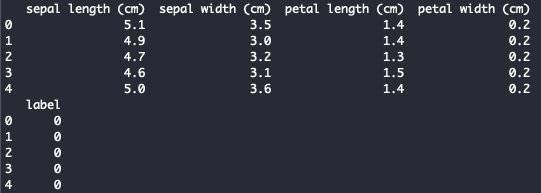
Fig. 3. Iris Dataset
Train test split:
# Split the data into training/testing sets
X_train = df_X[:-20]
X_test = df_X[-20:]

# Split the targets into training/testing sets
y_train = df_y[:-20]
y_test = df_y[-20:]
Initialize model and train:
# Create logistic regression object
regr = linear_model.LogisticRegression(solver='lbfgs', multi_class='multinomial')

# Train the model using the training sets
regr.fit(X_train, y_train)
Predict for test set:
# Make predictions using the testing set
y_pred = regr.predict(X_test)
Reference
[1] Andrew Ng Coursera: Machine Learning
[2] Scott Fortmann-Roe “Understanding the Bias-Variance Tradeoff”
Thank you for reading! See you in the next post!