
Linear Regression
Linear regression is one of the most basic learning algorithms in machine learning. At the same time, it is very important because it introduces concepts such as gradient descent and cost functions, which are used in most machine learning models. Hence, it is very important to understand the mechanics behind linear regression.
- What is linear regression?
- Hypothesis
- Cost function
- Gradient Descent
- Local Minimum vs Global Minimum
- Linear Regression with Scikit-Learn
- Reference
What is linear regression?
Linear regression is a supervised learning algorithm that predicts a real-valued output based on input values. Univariate linear regression refers to a linear regression with only one variable. Multivariate linear regression refers to a linear regression with more than one variables.
Hypothesis
The objective of a linear regression is to learn a function that predicts the dependent variable.
This hypothesis is typically represented by the following function:
\[\begin{align} &\text{h}_\theta(x) = \theta_0 + \theta_1(x_1) \ldots + \theta_n(x_n) \end{align}\]where
- \(x\) is the independent variables
- \(\theta\) is the optimized parameters for each independent variable
Cost function
A cost function measures the prediction accuracy of the hypothesis. For linear regression, a common cost function is the \(\textit{mean squared error}\), which calculates the average squared distances between the predicted values and actual values.
\[\begin{align} J(\theta_0,\ \ldots,\ \theta_n) = \frac{1}{m} \sum\limits_{i=1}^m (\text{h}_\theta(x^i) - y^i ) \end{align}\]where
- \(n\) is the number of independent variables
- \(m\) is the number of training examples
The overall objective is to minimise the cost function by iterating through different values of \(\theta\). The lowest possible value of the cost function is also known as the global minimum. The final linear regression model will hold the values of \(\theta\) that yields the lowest cost function.
\[\begin{align} \underset{\theta_0,\ \ldots,\ \theta_n}{\min} J(\theta_0,\ \ldots,\ \theta_n) \end{align}\]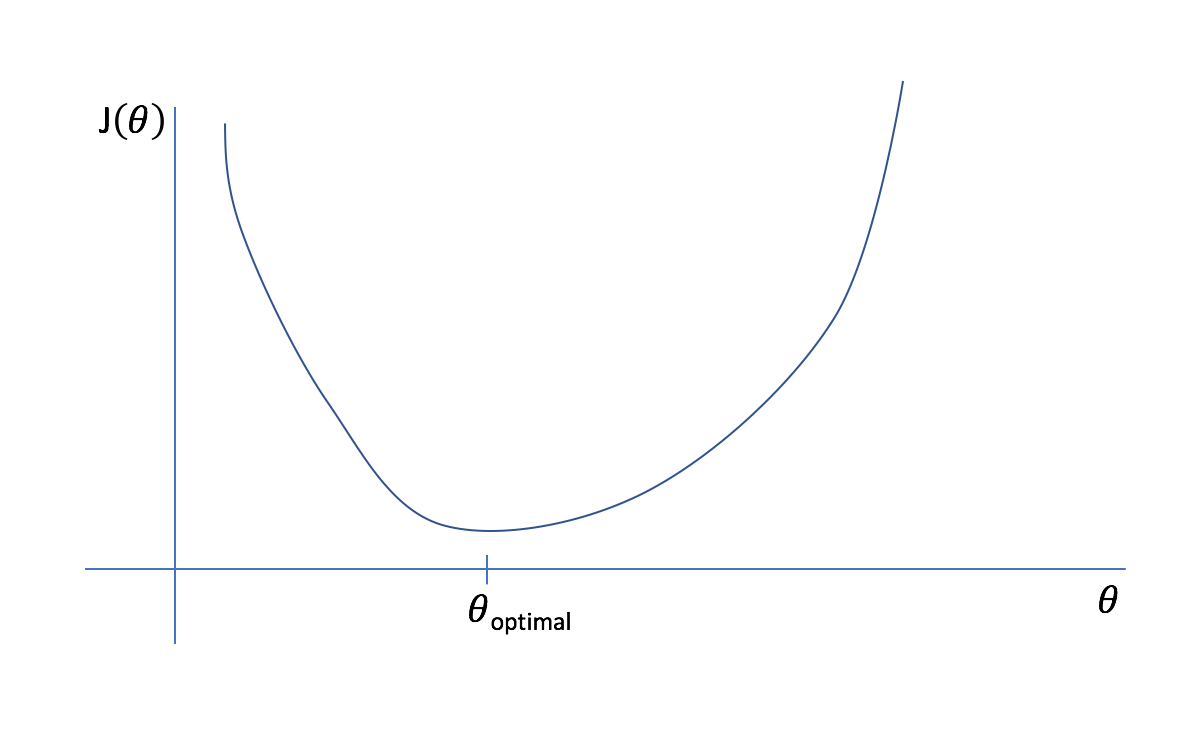
Fig. 1. 2-D Plot of Cost Function with One Variable - (Image source: here)
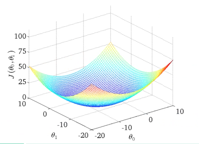
Fig. 2. 3-D Plot of Cost Function with Two Variables - (Image source: here)
Gradient Descent
Gradient descent is an algorithm used to estimate the parameters required to minimize the cost function.
Typically, gradient descent starts with randomly initialized values of \(\theta\). After which, \(\theta\) is being updated iteratively using gradient descent untill the cost function \(J(\theta_0,\ \ldots,\ \theta_n)\) ends up at a minimum.
The gradient descent algorithm is as follows:
\[\begin{align} \text{repeat until convergence} \ \left \{ \theta_j := \theta_j - \alpha \frac{\partial}{\partial \theta_j} J(\theta_0,\ \ldots,\ \theta_n) \right \}\\ \end{align}\]where
- values of \(j = 0, 1,\ \ldots,\ n\)
- \(\alpha\) is the learning rate
Each value of \(\theta\) is simultaneously updated using gradient descent untill the cost function stops decreasing.
To correctly implement simultaneous update, it is important to calculate all values of \(\theta\) before updating the new values of \(\theta\).
Correct implementation of simultaneous update:
\[\text{temp}_0 := \theta_0 - \alpha \frac{\partial}{\partial \theta_0} J(\theta_0,\ \ldots,\ \theta_n) \\ \text{temp}_1 := \theta_1 - \alpha \frac{\partial}{\partial \theta_1} J(\theta_0,\ \ldots,\ \theta_n) \\ ... \\ \text{temp}_n := \theta_n - \alpha \frac{\partial}{\partial \theta_n} J(\theta_0,\ \ldots,\ \theta_n) \\ \theta_0 := \text{temp}_0 \\ \theta_1 := \text{temp}_1 \\ ... \\ \theta_n := \text{temp}_n\]Wrong implementation of simulataneous update:
\[\text{temp}_0 := \theta_0 - \alpha \frac{\partial}{\partial \theta_0} J(\theta_0,\ \ldots,\ \theta_n) \\ \theta_0 := \text{temp}_0 \\ \text{temp}_1 := \theta_1 - \alpha \frac{\partial}{\partial \theta_1} J(\theta_0,\ \ldots,\ \theta_n) \\ \theta_1 := \text{temp}_1 \\ ... \\ \text{temp}_n := \theta_n - \alpha \frac{\partial}{\partial \theta_n} J(\theta_0,\ \ldots,\ \theta_n) \\ \theta_n := \text{temp}_n\]By taking the derivative of the cost function, we can find out which direction to move in order to reduce the cost function. The size of each step is determined by the learning rate \(\alpha\).
To understand this concept, suppose we have a cost function \(J(\theta_0)\) with just one parameter to optimize.
If \(\theta\) is more than the optimal value of \(\theta\) (at the global minimum), then the derivative of the cost function with be positive. Hence the value of \(\theta\) will be updated by subtracting a positive number. This ensures that the new \(\theta\) is lower in value.
In contrast, if \(\theta\) is less than the optimal value of \(\theta\), then the value of \(\theta\) will be updated by adding a positive number, ensuring that the new \(\theta\) is larger in value.
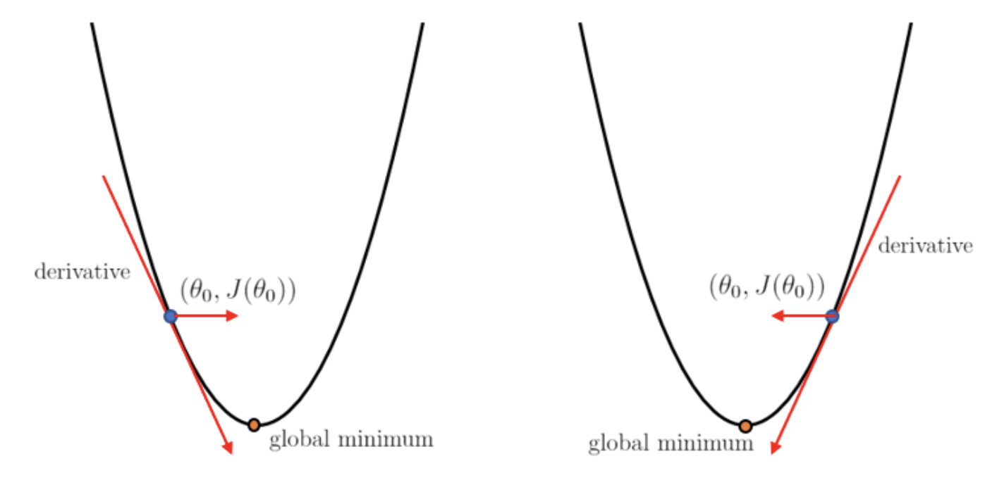
Fig. 3. Gradient Descent - (Image source: here)
However, this does not always ensure that \(\theta\) converges. If the learning rate is too large, the updated value of \(\theta\) might go beyond the optimal value of \(\theta\) at the global minimum.
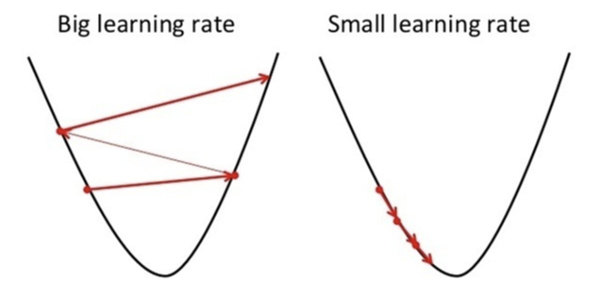
Fig. 4. Importance of Learning Rate - (Image source: here)
Local Minimum vs Global Minimum
Even when the values of \(\theta\) converges, we need to be aware that the cost function might not be at the global minima. That is, there could be another combination of \(\theta\) values where the value of cost function is even lower. This means that the values of \(\theta\) is stuck at a local minima.
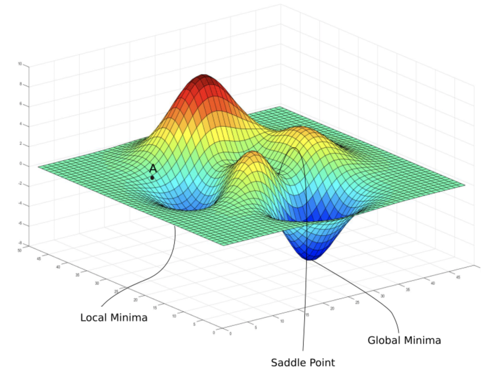
Fig. 5. Local Vs Global Minima - (Image source: here)
To solve this problem many different methods of gradient descent have been explored and created in order to allow the algorithm to escape from the local minima to reach a better minimum. One of the popular variants of gradient descent is \(\textit{stochastic gradient descent}\) which I will cover in more details in the future.
Linear Regression with Scikit-Learn
Implementing Linear Regression is pretty straight forward and can be implemented in a few lines of codes.
Begin by cloning my blog repository:
git clone https://github.com/wngaw/blog.git
In this problem, we are trying to predict the diabetes indicator given several features of an individual.
Now let’s install the relevant packages:
cd linear_regression_example/src
pip install -r requirements.txt
Import the relevant packages:
import pandas as pd
from sklearn import datasets, linear_model
from sklearn.metrics import mean_squared_error, r2_score
Import dataset:
# Load the diabetes dataset
diabetes = datasets.load_diabetes()
diabetes_X = diabetes.data
diabetes_y = diabetes.target
features = diabetes.feature_names

# Convert to Dataframe
df_X = pd.DataFrame(data=diabetes_X, columns=features)
df_y = pd.DataFrame(data=diabetes_y, columns=['diabetes_indicator'])
View dataset:
print(df_X.head())
print(df_y.head())
You should see this:
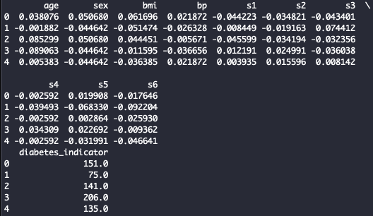
Fig. 6. Diabetes Dataset
Train test split:
# Split the data into training/testing sets
X_train = df_X[:-20]
X_test = df_X[-20:]

# Split the targets into training/testing sets
y_train = df_y[:-20]
y_test = df_y[-20:]
Initialize model and train:
# Create linear regression object
regr = linear_model.LinearRegression()

# Train the model using the training sets
regr.fit(X_train, y_train)
Predict for test set:
# Make predictions using the testing set
y_pred = regr.predict(X_test)
Evaluate model:
# The coefficients
print('Coefficients of features')
print(features)
print(regr.coef_)

# The mean squared error
print("Mean squared error: %.2f"
      % mean_squared_error(y_test, y_pred))

# Explained variance score: 1 is perfect prediction
print('Variance score: %.2f' % r2_score(y_test, y_pred))
You should see this:
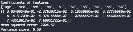
Fig. 7. Linear Regression Evaluation
Reference
[1] Andrew Ng Coursera: Machine Learning
Thank you for reading! See you in the next post!