
Field-aware Factorization Machines with xLearn
Recently, I discovered xLearn which is a high performance, scalable ML package that implements factorization machines (FM) and field-aware factorization machines (FFM). The first version of xLearn was released about 1 year ago as of writing.
![]()
FM was initially introduced and popularised by Steffen Rendle after winning 4th positions in both tracks in KDD cup 2012.
FM is a supervised learning algorithm that can be used for regression, classifications, and ranking. They are non-linear in nature and are trained using stochastic gradient descent (SGD).
FFM was later introduced and further improves FM. It was then used to win the 1st prize of three CTR competitions hosted by Criteo, Avazu, Outbrain, and also the 3rd prize of RecSys Challenge 2015.
To understand FM and FFM, we need to first understand a logistic regression model and a Poly2 model.
✅ Before jumping into Field-aware Factorization Machines, we need to first understand a logistic regression model, a Poly2 mode, and a Factorization Machines Model.
- Context
- The Optimization Problem
- Logistic Regression
- Degree-2 Polynomial Mappings (Poly2)
- Factorization Machines
- Field-aware Factorization Machines
- Field-aware Factorization Machines with xLearn
- Reference
Context
Assume we have the following dataset where we want to predict Clicked outcome using Publisher, Advertiser, and Gender:
| Dataset | Clicked | Publisher | Advertiser | Gender |
|---|---|---|---|---|
| TRAIN | YES | ESPN | NIKE | MALE |
| TRAIN | NO | NBC | ADIDAS | MALE |
The Optimization Problem
The model \(\pmb{w}\) for logistic regression, Poly2, FM, and FFM, is obtained by solving the following optimization problem:
\[\underset{\pmb{w}}{\min} \ \ \frac{\lambda}{2} \left\|\pmb{w} \right\|^{2} + \sum\limits_{i=1}^m log(1 + exp(-y_{i}\phi(\pmb{w}, \pmb{x_i}))\]where
- dataset contains \(m\) instances \((y_{i}, \pmb{x_i})\)
- \(y_i\) is the label and \(\pmb{x_i}\) is a n-dimensional feature vector
- \(\lambda\) is a regularization parameter
- \(\phi(\pmb{w}, \pmb{x})\) is the association between \(\pmb{w}\) and \(\pmb{x}\)
Logistic Regression
A logistic regression estimates the outcome by learning the weight for each feature.
For logistic regression,
\[\phi(\pmb{w}, \pmb{x}) = w_0 + \sum\limits_{i=1}^n w_i x_i\]where
- \(w_0\) is the global bias
- \(w_i\) is the strength of the i-th variable
In our context,
\[\begin{align} &\ \phi(\pmb{w}, \pmb{x}) = \\ &\ w_0 + \\ &\ w_{ESPN}x_{ESPN} + \\ &\ w_{NIKE}x_{NIKE} + \\ &\ w_{ADIDAS}x_{ADIDAS} + \\ &\ w_{NBC}x_{NBC} + \\ &\ w_{MALE}x_{MALE} \end{align}\]However, logistic regression only learns the effect of each features individually rather than in a combination.
Degree-2 Polynomial Mappings (Poly2)
A Poly2 model captures this pair-wise feature interaction by learning a dedicated weight for each feature pair.
For Poly2,
\[\phi(\pmb{w}, \pmb{x}) = w_0 + \sum\limits_{i=1}^n w_i x_i + \sum\limits_{i=1}^n \sum\limits_{j=i + 1}^n w_{h(i, j)} x_i x_j\]In our context,
\[\begin{align} &\ \phi(\pmb{w}, \pmb{x}) = \\ &\ w_0 + \\ &\ w_{ESPN}x_{ESPN} + \\ &\ w_{NIKE}x_{NIKE} + \\ &\ w_{ADIDAS}x_{ADIDAS} + \\ &\ w_{NBC}x_{NBC} + \\ &\ w_{MALE}x_{MALE} + \\ &\ w_{ESPN, NIKE}x_{ESPN}x_{NIKE} + \\ &\ w_{ESPN, MALE}x_{ESPN}x_{MALE} + \\ &\ ... \end{align}\]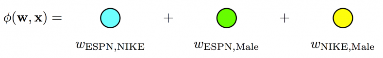
Fig. 1. Poly2 model - A dedicated weight is learned for each feature pair (linear terms ignored in diagram) (Image source: here)
However, a Poly2 model is computationally expensive as it requires the computation of all feature pair combinations. Also, when data is sparse, there might be some unseen pairs in the test set.
Factorization Machines
FM solves this problem by learning the pairwise feature interactions in a latent space. Each feature has an associated latent vector. The interaction between two features is an inner-product of their respective latent vectors.
For FM,
\[\phi(\pmb{w}, \pmb{x}) = \textit{w}_{0} + \sum\limits_{i=1}^n w_i x_i + \sum\limits_{i=1}^n \sum\limits_{j=i + 1}^n \langle \mathbf{v}_{i} \cdot \mathbf{v}_{j} \rangle x_i x_j\]where
- \[\langle \mathbf{v}_{i}, \mathbf{v}_{j} \rangle := \sum\limits_{f=1}^k v_{i,f} \cdot v_{j,f}\]
- \(k \in \mathbb{N}^{+}\) is the hyperparameter that defines the dimensionality of the vectors
In our context,
\[\begin{align} &\ \phi(\pmb{w}, \pmb{x}) = \\ &\ w_0 + \\ &\ w_{ESPN}x_{ESPN} + \\ &\ w_{NIKE}x_{NIKE} + \\ &\ w_{ADIDAS}x_{ADIDAS} + \\ &\ w_{NBC}x_{NBC} + \\ &\ w_{MALE}x_{MALE} + \\ &\ \langle \textbf{v}_{ESPN, k} \cdot \textbf{v}_{NIKE, k} \rangle x_{ESPN} x_{NIKE} + \\ &\ \langle \textbf{v}_{ESPN, k} \cdot \textbf{v}_{MALE, k} \rangle x_{ESPN} x_{MALE} + \\ &\ \langle \textbf{v}_{NIKE, k} \cdot \textbf{v}_{MALE, k} \rangle x_{NIKE} x_{MALE} + \\ &\ ... \end{align}\]where
\[\begin{align} &\ \langle \textbf{v}_{ESPN, k} \cdot \textbf{v}_{NIKE, k} \rangle = \\ &\ v_{ESPN, 1} * v_{NIKE,1} + \\ &\ v_{ESPN, 2} * v_{NIKE,2} + \\ &\ v_{ESPN, 3} * v_{NIKE,3} + \\ &\ ... \\ &\ v_{ESPN, k} * v_{NIKE,k} \end{align}\]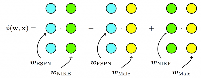
Fig. 2. Factorization Machines - Each feature has one latent vector, which is used to interact with any other latent vectors (linear terms ignored in diagram) (Image source: here)
| Dataset | Clicked | Publisher | Advertiser | Gender |
|---|---|---|---|---|
| TRAIN | YES | ESPN | NIKE | MALE |
| TRAIN | NO | NBC | ADIDAS | MALE |
| TEST | YES | ESPN | ADIDAS | MALE |
In the case of unseen pairs in the test set (ESPN, ADIDAS) and (ADIDAS, MALE), a reasonable estimation can still be predicted since FM is able to learn \(w_ESPN\) from (ESPN, NIKE) and \(w_ADIDAS\) from (NBC, ADIDAS).
For Poly 2, there is no way to learn the weights of \(w_{ESPN, ADIDAS}\) or \(w_{ADIDAS, MALE}\).
libFM by Steffen Rendle is an open-sourced software, and it can be found here.
However, the latent effect between publisher and advertisers (P X A) may be different from the latent effect between publishers and gender (P X G). Hence, the \(w_ESPN\) used should be specific to the field that it is paired with.
Field-aware Factorization Machines
FFM addresses this issue by splitting the original latent space into smaller latent spaces specific to the fields of the features.
For FFM,
\[\phi(\pmb{w}, \pmb{x}) = w_0 + \sum\limits_{i=1}^n w_i x_i + \sum\limits_{i=1}^n \sum\limits_{j=i + 1}^n \langle \mathbf{v}_{i, f_{2}} \cdot \mathbf{v}_{j, f_{1}} \rangle x_i x_j\]where
- \(f_1\) and \(f_2\) are respective fields of \(i\) and \(j\)
Since each latent vector only needs to learn the field specific effect, a smaller dimension \(k\) is needed (\(k_{FFM} \ll k_{FM}\)).
In our context, we split
- \(w_ESPN\) into \(w_{ESPN, PUBLISHER}\) and \(w_{ESPN, GENDER}\)
- \(w_NIKE\) into \(w_{NIKE, ADVERTISER}\) and \(w_{NIKE, GENDER}\)
- \(w_MALE\) into \(w_{MALE, PUBLISHER}\) and \(w_{MALE, ADVERTISER}\)
Therefore,
\[\begin{align} &\ \phi(\pmb{w}, \pmb{x}) = \\ &\ w_0 + \\ &\ w_{ESPN}x_{ESPN} + \\ &\ w_{NIKE}x_{NIKE} + \\ &\ w_{ADIDAS}x_{ADIDAS} + \\ &\ w_{NBC}x_{NBC} + \\ &\ w_{MALE}x_{MALE} + \\ &\ \langle \textbf{v}_{ESPN, ADVERTISER, k} \cdot \textbf{v}_{NIKE, PUBLISHER, k} \rangle x_{ESPN} x_{NIKE} + \\ &\ \langle \textbf{v}_{ESPN, GENDER, k} \cdot \textbf{v}_{MALE, PUBLISHER, k} \rangle x_{ESPN} x_{MALE} + \\ &\ \langle \textbf{v}_{NIKE, GENDER, k} \cdot \textbf{v}_{MALE, ADVERTISER, k} \rangle x_{NIKE} x_{MALE} + \\ &\ ... \end{align}\]where
\[\begin{align} &\ \langle \textbf{v}_{ESPN, ADVERTISER, k} \cdot \textbf{v}_{NIKE, PUBLISHER, k} \rangle = \\ &\ v_{ESPN, ADVERTISER, 1} * v_{NIKE, PUBLISHER, 1} + \\ &\ v_{ESPN, ADVERTISER, 2} * v_{NIKE, PUBLISHER, 2} + \\ &\ v_{ESPN, ADVERTISER, 3} * v_{NIKE, PUBLISHER, 3} + \\ &\ ... \\ &\ v_{ESPN, ADVERTISER, k} * v_{NIKE, PUBLISHER, k} \end{align}\]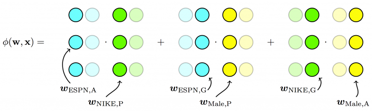
Fig. 3. Field-aware Factorization Machines - Each feature has several latent vectors, one of them is used depending on the field of the other feature (linear terms ignored in diagram) (Image source: here)
libFFM is open sourced, and can be found here.
Field-aware Factorization Machines with xLearn
Implementing FFM is pretty straight forward and can be implemented in a few lines of codes.
Begin by cloning my blog repository:
git clone https://github.com/wngaw/blog.git
In this problem, we are trying to predict the loan status (approve/reject) of a mortgage loan given several features of it.
Now let’s install the relevant packages:
cd xlearn_example/src
pip install -r requirements.txt
Import the relevant packages, helper function, and config file:
import pandas as pd
import xlearn as xl
from sklearn.model_selection import train_test_split
from utils import _convert_to_ffm
import config
import warnings
warnings.filterwarnings('ignore')
Note: _convert_to_ffm is a user-defined function that encodes your train set data frame into libffm format that is a requirement for FFM to work.
Import train dataset:
train = pd.read_csv('data/train.csv')
Some pre-processing:
cols = ['Education','ApplicantIncome','Loan_Status','Credit_History']
train_sub = train[cols]
train_sub['Credit_History'].fillna(0, inplace = True)
dict_ls = {'Y':1, 'N':0}
train_sub['Loan_Status'].replace(dict_ls, inplace = True)
Splitting into train and test:
train, test = train_test_split(train_sub, test_size = 0.3, random_state = 5)
Checking our train set:
print(f' train data: \n {X_train.head()}')
You should see this:
| Education | ApplicantIncome | Loan_Status | Credit_History |
|---|---|---|---|
| Not Graduate | 3596 | 1 | 0 |
| Graduate | 7740 | 1 | 1 |
| Graduate | 3158 | 1 | 1 |
| Graduate | 6000 | 1 | 0 |
| Graduate | 4566 | 0 | 1 |
Initialize encoder:
encoder = {"currentcode": len(config.NUMERICAL_FEATURES),
           "catdict": {},
           "catcodes": {}}
Note:
- currentcode = Unique index for each numerical field or categorical variables
- catdict = Dictionary that stores numerical and categorical variables
- catcodes = Dictionary that stores index for each categorical variables per categorical field
Start encoding your data frames into libffm format:
encoder = _convert_to_ffm('data/', train, 'train', config.GOAL[0],
                          config.NUMERICAL_FEATURES,
                          config.CATEGORICAL_FEATURES,
                          config.ALL_FEATURES,
                          encoder)

encoder = _convert_to_ffm('data/', test, 'test', config.GOAL[0],
                          config.NUMERICAL_FEATURES,
                          config.CATEGORICAL_FEATURES,
                          config.ALL_FEATURES,
                          encoder)
Note: your encoded data will be saved under data as train_ffm.txt and test_ffm.txt
Start training:
ffm_model = xl.create_ffm()
ffm_model.setTrain("data/train_ffm.txt")
ffm_model.setValidate("data/test_ffm.txt")
param = {'task': 'binary',
         'lr': 0.2,
         'lambda': 0.002,
         'metric': 'auc'}
ffm_model.fit(param, 'trained_models/model.out')
You should see this:
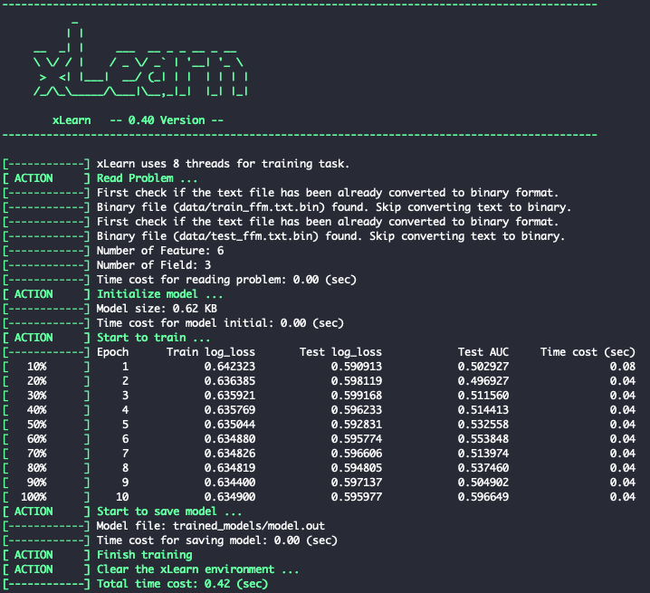
Fig. 4.Training xLearn Model
Note: your trained model will be stored under trained_models as model.out
To perform cross_validation:
ffm_model = xl.create_ffm()
ffm_model.cv(param)
You should see this:
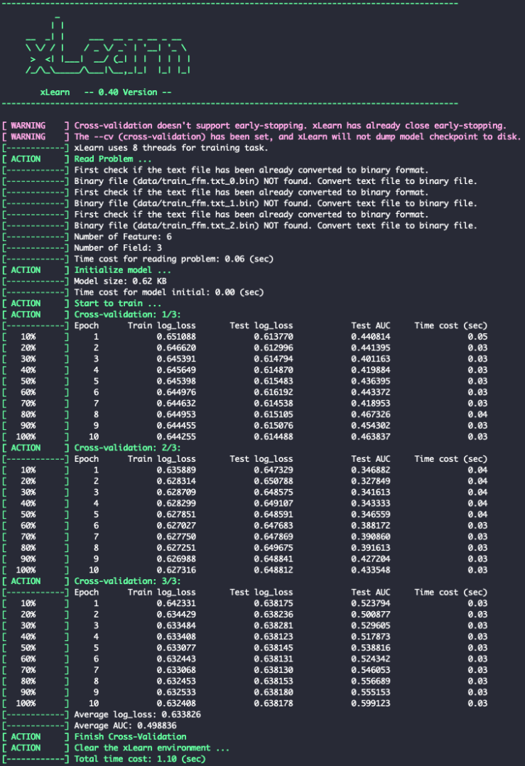
Fig. 5. xLearn Cross-Validation
Let’s start predicting!
ffm_model.setTest("data/test_ffm.txt")
ffm_model.setSigmoid()
ffm_model.predict("trained_models/model.out", "output/predictions.txt")
Note:
- prediction probability will be stored under output as predictions.txt
- you can convert the score to binary by using ffm_model.setSign() instead of ffm.mode.setSigmoid()
To perform online learning on new dataset:
ffm_model = xl.create_ffm()
ffm_model.setTrain("data/train_ffm.txt")
ffm_model.setValidate("data/test_ffm.txt")
ffm_model.setPreModel("trained_models/model.out")
param = {'task': 'binary', 'lr': 0.2, 'lambda': 0.002}
ffm_model.fit(param, "trained_models/model.out")
You should see this:
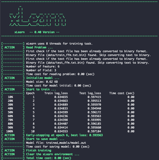
Fig. 6. xLearn Online Learning
Reference
[1] Steffen Rendle “Factorization Machines” ICDM. 2010.
[2] Yuchin Juan et al. “Field-aware Factorization Machines for CTR Prediction” ACM Conference on Recommender Systems. 2016.
[3] Yuchin Juan et al. “Field-aware Factorization Machines in a Real-world Online Advertising System” International Conference on World Wide Web Companion. 2017.
[4] Yuchin Juan “CTR Prediction: From Linear Models to Field-aware Factorization Machines”
[5] Ankit Choudhary “Introductory Guide – Factorization Machines & their application on huge datasets”
Thank you for reading! See you in the next post!